GLG410/598--Computers in Earth and Space Exploration
Lecture 5
Introduction
Today's lecture will focus on some tools that you can use to explore your dataset a little more closely.
Along the way, we will teach you two important concepts that we use heavily in data analysis.
First we will go over some syntax that will help you construct some special arrays very quickly.
Then we will introduce the find function in Matlab that helps you search for values in your data.
For the remaining class time, you will be able to use these tools to create several different kinds of plots in Matlab.
Array Construction
Several different kinds of plots require use to temporarily make our own "data".
For example, you may have found this out when creating your histogram.
The second argument in the hist function is an array of numbers that defines your center of each bin.
For a histogram of number of earthquakes per year, this function requires us to make an array that contained each year from 1973 through 2009.
You can either create this vector of number by:
>> Years = [1973 1974 1975 1976 1977 1978 1979 ...
    1980 1981 1982 1983 1984 1985 1986 1987 1988 1989 ...
    1990 1991 1992 1993 1994 1995 1996 1997 1998 1999 ...
    2000 2001 2002 2003 2004 2005 2006 2007 2008 2009];
Or, you can define a vector by using the following syntax:
min_value:increment:max_value
Use it like this example:
>> Years = [1973:1:2009];
But what if you don't know the minimum and maximum values to use? Here is how I might make my vector by using the min and max functions:
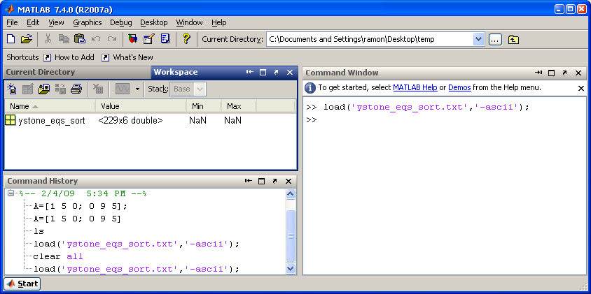
>> MinYear = min(ystone_eqs_sort(:,1));
>> MaxYear = max(ystone_eqs_sort(:,1));
>> Years = [MinYear:1:MaxYear];
Even better, you can insert the min and max functions directly into the vector creation line:
>> Years = [min(ystone_eqs_sort(:,1)):1:max(ystone_eqs_sort(:,1))];
Some other specialized arrays that you can make:
A Square Matrix with all 1's
>> ones(3)

ans =
    1    1    1
    1    1    1
    1    1    1
A Square Matrix with all 0's
>> zeros(3)

ans =
    0    0    0
    0    0    0
    0    0    0
To make arrays with n rows and m columns, the syntax would be ones(n,m) and zeros(n,m).
HINT: Use these ones and zeros functions in combination with multiplication or addition to make arrays of other numbers
Example:
>> 17.2 .* ones(4,1)

ans =
    17.2
    17.2
    17.2
    17.2
Dataset Subsetting
Recall Lecture 3.
Let's step back for a moment and talk about how to find some parts of this array that satisfy a criterion:
>> A=[1 5 0; 0 9 5]

A =

     1     5     0
     0     9     5

>> tf = A > 5

tf =

     0     0     0
     0     1     0
In the above example, tf is a new matrix filled with 1's and 0's.
There is a 1 where the conditional of A > 5 was true, and 0 where it was false.
How about
>> tf = A >= 5

tf =

     0     1     0
     0     1     1
or
>> tf = A < 5

tf =

     1     0     1
     1     0     0

>> tf = A == 5

tf =

     0     1     0
     0     0     1
Note in the latter case, the use of the == to mean the test if they are equal and how that varies from the single = which is the assignment of the result to the tf variable.
Let's go back to:
>> A

A =

     1     5     0
     0     9     5

>> tf = A > 5

tf =

     0     0     0
     0     1     0
Now here is where things get to be really neat:
>> locs = find(tf)

locs =

     4

>> A(locs)

ans =

     9
Look at the MATLAB documentation for find.
Basically it returns the array locations where values are == 1.
In combination with the conditional or boolean statement like the tf examples above, it is very powerful for processing data.
Let's apply to the Yellowstone data:
Let's find all the events that are in 2008:
>> tf=ystone_eqs_sort(:,1)==2008;
>> locs=find(tf)
Now let's plot them:
>> figure(1)
>> clf
>> plot(ystone_eqs_sort(:,4),ystone_eqs_sort(:,3), 'k.')
>> hold on
>> plot(ystone_eqs_sort(locs,4),ystone_eqs_sort(locs,3), 'ro')
>> xlabel('longitude')
>> ylabel('latitude')
>> title('Yellowstone seismicity (2008 in red)')

A bit about figure(1), clf, and hold on:
figure is a command used to initialize a new figure window.
If you just type it in, it will display and empty figure window.
Typing figure(1) makes the window "Figure 1" the current figure window.
Yes, you can have multiple figure windows open at the same time.
Typing figure(2) would make the window "Figure 2" current, and so on.
So any plotting commands used subsequently will be displayed in the current figure window.
clf will clear the current figure window of all plots that are in it.
hold on is a VERY useful function to learn when making plots.
As in the previous example, we wanted to first plot all the earthquakes.
Then, we wanted to "overlay" circles around the 2008 events.
If we were to type:
>> plot(ystone_eqs_sort(:,4),ystone_eqs_sort(:,3), 'k.')
>> plot(ystone_eqs_sort(locs,4),ystone_eqs_sort(locs,3), 'ro')
the second plot command would "blow away" the first earthquakes that we plotted.
So hold on, tells Matlab to "hold on! We've got some more stuff to plot here!"
To then release the figure, so that the next plot command will replace the figure, we can type hold off.
In-Class Work
We can now work on building up your Matlab plotting toolbox by exploring the Yellowstone data a little more.
Choose at least one other plot type and explore some of the features within the dataset.
Here is a list of possible selections to help guide your creative thinking:
- Earthquake locations: color coded by year
HINT: you may want to explore isolating individual years of peak activity
- Earthquake locations: color coded by depth
- Earthquake locations: color coded by magnitude
- Magnitude vs. depth
- Magnitude histogram
- 3D Earthquake locations: latitude/longitude/depth
HINT: use the plot3 function
BE SURE TO USE THE MATLAB HELP TO FIND PROPER SYNTAX AND USAGE FOR FUNCTIONS!
These are not the only choices, so we encourage you to try things on your own.
GLG410/598 Computers in Earth and Space Exploration
Last modified: February 4, 2009