GLG410/598--Computers in Earth and Space Exploration
Lecture 6: Graphical Interaction with Plots and Subsetting
ginput, gtext, and find
Today's lecture will continue a discussion of tools for exploring your data.
Set up the example
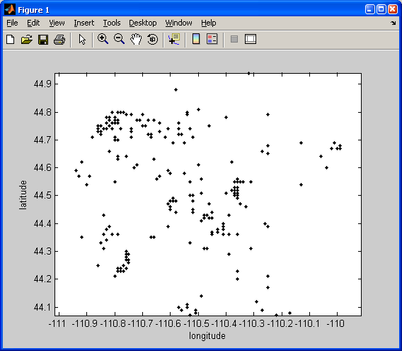
Let's go back to our Yellowstone seismicity data.
I am going to load the data, set up a few variables, and then plot it:
load('ystone_eqs_sort.txt','-ascii');
year = ystone_eqs_sort(:,1);
x_locations = ystone_eqs_sort(:,4);
y_locations = ystone_eqs_sort(:,3);
depth = ystone_eqs_sort(:,5);
magnitudes = ystone_eqs_sort(:,6);

figure(1)
clf
plot(x_locations,y_locations,'k.')
xlabel('longitude')
ylabel('latitude')
axis equal
Getting the locations of mouse clicks on a plot
Say you want to have the user select some portion of the data interactively using the mouse. You can get the coordinates of a user's clicks by using the Matlab command ginput.
I added this code to my script so that you can tell the user what to do:
fprintf(1, 'click on lower left and upper right of the area of interest\n')
Note that the \n
means "add a new line after this."
NOTE: fprintf is a function that is used to write out text (to a file or the command window).
The "1" as the first argument in fprintf tells the function to print the text to the screen.
The script entry looks like this:
[X,Y] = ginput(2);

xmin=min(X)
xmax=max(X)
ymin=min(Y)
ymax=max(Y)
The argument of 2 to ginput tells it to take two clicks. When you move the mouse over the figure, you will see that the cursor turns into a moving cross hair:
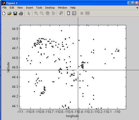 The result in that case is:
click on lower left and upper right of the area of interest
xmin =

 -110.4103


xmax =

 -110.2831


ymin =

   44.4732


ymax =

   44.5826
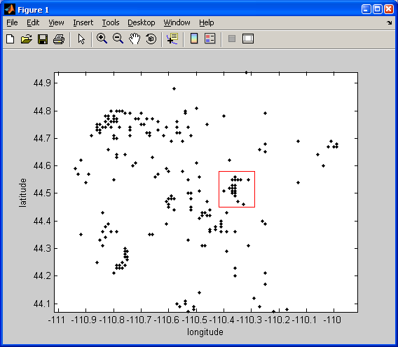
Let's draw a red box then around that selection:
%this draws a box. Realize that it has 5 vertices because you have to close it back around to the beginning
xs = [xmin xmax xmax xmin xmin];
ys = [ymin ymin ymax ymax ymin];

hold on
plot(xs, ys, 'r-')
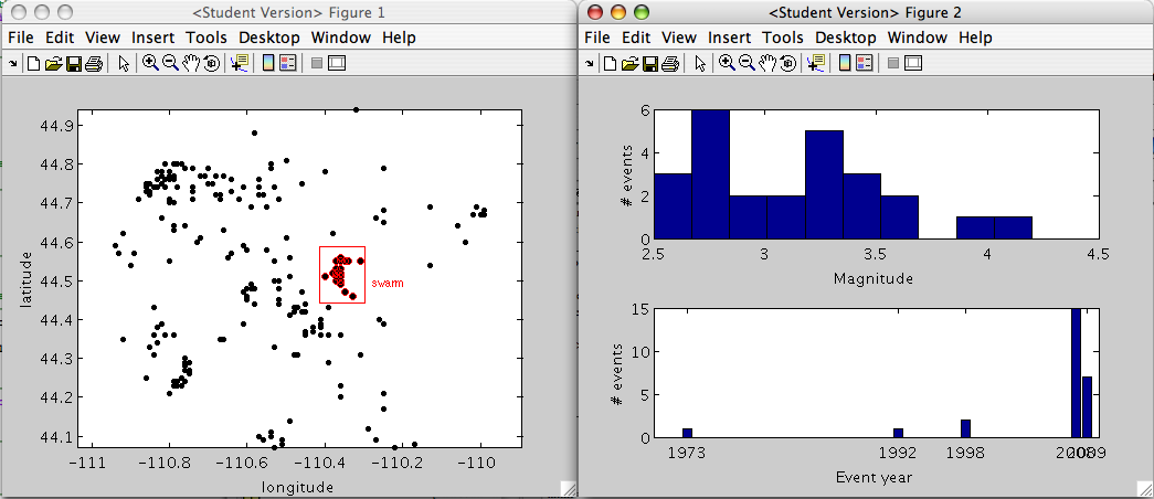
Finding the events within a user-defined box
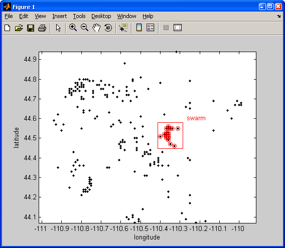
Now for some real interactivity. Find the events inside that square:
t> tf = x_locations <= xmax & x_locations >= xmin & y_locations <= ymax & y_locations >= ymin;
locs = find(tf);
plot(x_locations(locs),y_locations(locs),'ro')
And, let me teach you about another useful interactive item: Matlab command gtext. This will let us label our box:
NOTE: input is a function that lets you write out a message or question to the screen and ask the user for input. The user can then type anything, and that input is then assigned to the variable specified by input. If you want to get really fancy, tryout the function inputdlg. This gives you a popup box to write your response.
your_label = input('What is your label for that selection? \n', 's');

gtext(your_label, 'Color', 'r')
I typed swarm
as the label at the command line.
Operations on the selection
Histograms of event year
figure(2)
clf
years_for_hist = unique(year(locs));

subplot(2,1,1)
hist(year(locs), years_for_hist);
xlabel('Event year')
ylabel('# events')
subplot(2,1,2)
n = hist(year(locs), years_for_hist);
bar(years_for_hist, n)
xlabel('Event year')
ylabel('# events')
Here I have introduced the concept of subplot.
By calling subplot we can place multiple axes into the same figure window and specify where in the window we want the axes to be plotted.
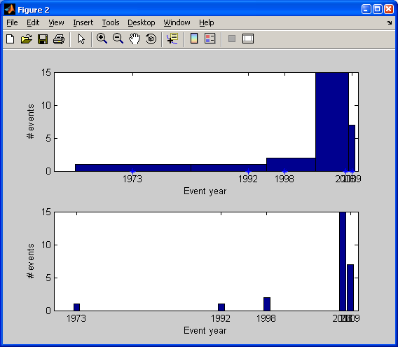
Which of the above did you like better? Do you see what was different?
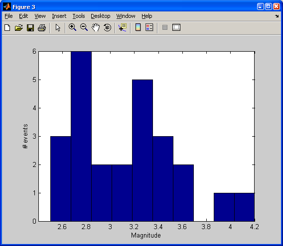
Histograms of event magnitude
figure(3)
clf
hist(magnitudes(locs))
xlabel('Magnitude')
ylabel('# events')
Our In-Class Modifications
String Concatenation
In our in-class discussions, we introduced of simple "concatenation" using the brackets. Just like you make a numeric vector:
>> [1 2]

ans =

    1    2
You can also concatinate strings (text):
>> ['My' 'String']

ans =

MyString
Our use of this in-class was to concantenate the letter that defined our box color with the symbol that defined the line connected box vertices:
>> color_label = 'r';
>> [color_label '-']

ans =

r-
Remeber that we used the input function to ask the user what color they wanted to make the box:
color_label = input('Click on lower left and upper right of the area of interest, and by thway, what color?\n', 's');
Then, we added the concatenation that we discussed above to our plot command for drawing the box:
plot(xs, ys, [color_label '-'])
Then, we added the concatenation to our plot command for adding circles around our "swarm earthquakes":
plot(x_locations(locs),y_locations(locs),[color_label 'o'])
Finally, we also added the new color label to our "swarm" text:
gtext(your_label, 'Color', color_label)
Replacing the "bad" event histogram with the magnitude histogram
We also decided that the top event histogram didn't look as good as our bottom event histogram where we used the bar command.
Because of that we decided to replace what was in subplot(2,1,1) with our magnitude histogram:
subplot(2,1,1)
hist(magnitudes(locs))
xlabel('Magnitude')
ylabel('# events')

subplot(2,1,2)
n = hist(year(locs), years_for_hist);
bar(years_for_hist, n)
xlabel('Event year')
ylabel('# events')
GLG410/598 Computers in Earth and Space Exploration
Last modified: February 11, 2009