GLG410/598--Computers in Earth and Space Exploration
Lecture 7: simple looping and matrix construction
Assignment 4: Interactive Yellowstone Earthquake Analysis
For this assignment, please assemble the operations of Tuesday's interactive Yellowstone seismicity analysis.
Cut and paste the commands from the lecture into a Matlab m-file (script).
Include comments in the script that tell the user what each group of commands is doing.
Perform your analysis, including the histograms, on a couple of earthquake groups and compare.
Remember to save your maps and histograms using the print function.
Make sure you are not "overwriting" previous jpeg files when you analyze more than one swarm!
Build a web page for this assignment that contains the following:
- Map of event group 1
- Histograms for group 1 (earthquakes per year and earthquake magnitudes)
- Map of event group 2
- Histograms for group 2 (earthquakes per year and earthquake magnitudes)
- A link to your M-file (Matlab script) used to make these plots
- Discussion: Compare these groups of events using these graphs and describe what you see. Speculate briefly about the processes that might be operating in this system and why or why not the groups might be swarms/clusters.
Grading Rubric (30 points):
- Web page for the assignment--5 points
- Map and Histogram plots--5 points
- Matlab m-file (including comments)--10 points
- Discussion--10 points
Assignment is due Tuesday, February 17, 2009.
Introduction
This lecture is our fist introduction to what is called "control flow" in programming. We will start out with For Loops to demonstrate how you can do many repetative tasks without explicitly writing each successive iteration.
For loops
Help on for loops can be found here.
Sometimes, you need go go through a data set to do some analysis and you cannot do it in the simple vector mode of Matlab.
For example,
>> for n = 1:5
n
end

n =

     1


n =

     2


n =

     3


n =

     4


n =

     5
Set up the example
Let's go back to our Yellowstone seismicity data.
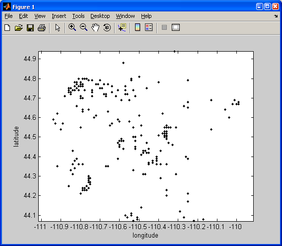
I am going to load the data, set up a few variables, and then plot it:
load('ystone_eqs_sort.txt','-ascii');
year = ystone_eqs_sort(:,1);
x_locations = ystone_eqs_sort(:,4);
y_locations = ystone_eqs_sort(:,3);
depth = ystone_eqs_sort(:,5);
magnitudes = ystone_eqs_sort(:,6);

figure(1)
clf
plot(x_locations,y_locations,'k.')
xlabel('longitude')
ylabel('latitude')
axis equal
hold on
One loop
stepsize = 0.1;
long_range=min(x_locations):stepsize:max(x_locations);
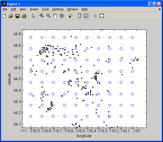
for long = long_range
plot(long,min(y_locations),'bo')
end
Here we need to specify the step size as we move across the grid. Notice the blue circles across the base:

Nested loops
stepsize = 0.1;
long_range=min(x_locations):stepsize:max(x_locations);
lat_range = min(y_locations):stepsize:max(y_locations);
for long = long_range
    for lat = lat_range
        plot(long,lat,'bo')
    end
end
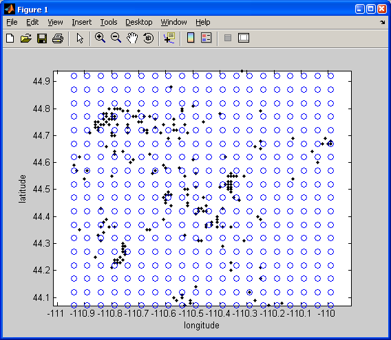
Here we need to moved across the study area in both the latitude and the longitude directions by the magnitude of the stepsize:
Here it is with a stepsize of 0.05:
Operations inside the nested loop
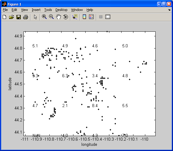
stepsize = 0.25;
long_range=min(x_locations):stepsize:max(x_locations);
lat_range = min(y_locations):stepsize:max(y_locations);
for long = long_range
    for lat = lat_range
       tf = x_locations <= long+stepsize./2 & x_locations >= long-stepsize./2 & y_locations <= lat+stepsize./2 & y_locations >= lat-stepsize./2;
       locations = find(tf);
       mean_depth = mean(depth(locations));
       s = sprintf('%2.1f',mean_depth);
       text(long, lat, s);
    end
end
In this example, I have searched for the depth values within each step (+/- half the step size from the lat long location of the estimate). Then, I computed their mean, converted the mean and some text to a string (sprintf), and plotted that amount using text.
3D Plots of Locations - plot3
We could also plot the locations in 3D using the earthquake depth column. Use the plot3 function:
figure(2)
plot3(x_locations,y_locations,-depth,'r.')
grid on
title('Yellowstone Earthquake Hypocenters')
xlabel('longitude')
ylabel('latitude')
zlabel('depth')
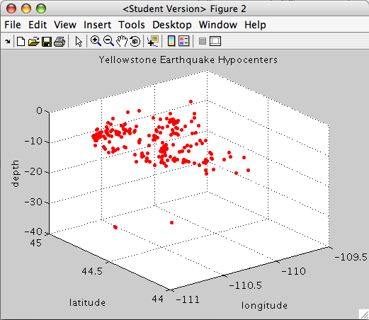
The grid on command is used to display the x,y,z grid in the background to give some perspective to the plot.
Scaled Images of Values in Matrices: using imagesc
We can also gather these values into a matrix that mimics our grid. Then we can plot the scaled values in that matrix using imagesc.
Repeat the last loop, but lets reference the numbers that we loop through in a little bit different way. We will also build out a matrix of our mean depth values.
stepsize = 0.1;
long_range=min(x_locations):stepsize:max(x_locations);
lat_range = min(y_locations):stepsize:max(y_locations);

% Here we are looping over the range of longitudes
for n = 1:length(long_range)

    % Here we are looping over the range of latitudes
    for m = 1:length(lat_range)

        % Notice that we have to index "long_range" by n and "lat_range" by m
        tf = x_locations <= long_range(n)+stepsize./2 & x_locations >= long_range(n)-stepsize./2 & y_locations <= lat_range(m)+stepsize./2 & y_locations >= lat_range(m)-stepsize./2;
        locations = find(tf);

        % Build the "mean_depth" matrix with rows = latitudes, columns = longitudes
        mean_depth(m,n) = mean(depth(locations));
    end
end
Notice some slight changes to our loop.
Lets plot the values of this matrix using imagesc.
The syntax is: imagesc(x,y,D)
This is how we would plot our data:
figure(3)
clf
imagesc(long_range,lat_range,mean_depth)
xlabel('longitude')
ylabel('latitude')
set(gca,'Ydir','normal')
colorbar
hold on
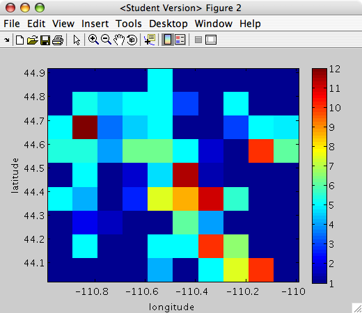
NOTE: The colorbar function will plot the color scale for the image. The set function is used to change Properties after you have plotted your data. Here we change the property, Ydir to plot the y-axis so that larger values are above smaller values. The first argument in set is gca, which tells the set command:"I want to set a property in the current axis (the axis you just plotted your data in)."
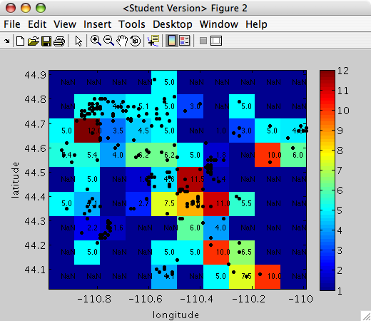
We can then plot the earthquakes over the image, along with the mean depth values in each box:
plot(x_locations,y_locations,'k.')
for n = 1:length(long_range)
    for m = 1:length(lat_range)
        s = sprintf('%2.1f',mean_depth(m,n));
        text(long_range(n), lat_range(m), s);
    end
end
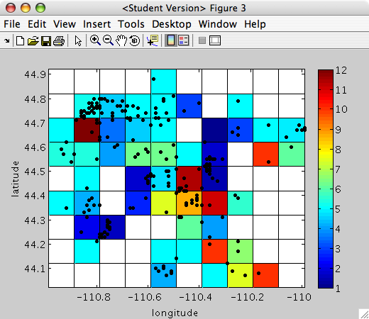
pcolor is similar to imagesc
If you notice the above figure plots grids where there is "no data" (NaN) as blue. This is a limitation of imagesc. The function pcolor plots a pseudocolor image of your matrix. This is very similar to a scaled image produced by imagesc. If you use this function, your "no data" blocks will now be white.
FIRST, we need to precondition our x-axis vector (long_range), y-axis vector (lat_range), and matrix (mean_depth). This is because pcolor plots the colors at the vertices (not the center of the grid like imagesc).
long_range = long_range - (stepsize./2);
lat_range = lat_range - (stepsize./2);
long_range_vert = [long_range (long_range(end)+stepsize)];
lat_range_vert = [lat_range (lat_range(end)+stepsize)];
mean_depth(end+1,:) = NaN .* ones(1,size(mean_depth,2));
mean_depth(:,end+1) = NaN .* ones(size(mean_depth,1),1);
Now we can plot the matrix by replacing imagesc by pcolor:
figure(4)
clf
pcolor(long_range_vert,lat_range_vert,mean_depth)
xlabel('longitude')
ylabel('latitude')
set(gca,'Ydir','normal')
colorbar
hold on
plot(x_locations,y_locations,'k.')
Assignment 5: Yellowstone Earthquake Analysis - Gridding and Image Plotting
For this assignment, assemble the operations of Thursday's tutorial of "for loops" and image plotting using the Yellowstone seismicity data.
Cut and paste the commands from the lecture into a Matlab m-file (script).
Include comments in the script that tell the user what each group of commands is doing.
Build a web page for this assignment that contains the following:
- (3D Plot) Plot 3D locations of earthquakes
- For 3 different resolutions (stepsize = 0.25 , 0.1, and 0.05)):
- (Grid Plot) Plot blue circles at each point in the grid on top of earthquake locations
- (Text Label Plot) Plot text labels for mean depths on top of earthquake locations
- (Scaled Image Plot) Plot scaled image (imagesc or pcolor) of mean depths below earthquake locations
- A link to your M-file (Matlab script) used to make these plots
- Discussion: relate the mean depth or variation in depth with the swarms, magnitudes, and other analysis from the prior assignment.
- Include a link to a web article on the ongoing swarm that you find particularly interesting. Note that this has been broadly mentioned in the popular media lately.
Grading Rubric (35 points):
- Web page for the assignment--3 points
- 3D Location Plot--3 points
- Grid Plots--3 points
- Text Label Plots--3 points
- Scaled Image Plots--3 points
- Matlab m-file (including comments)--10 points
- Discussion and link--10 points
Assignment is due Thursday, February 19, 2009.
GLG410/598 Computers in Earth and Space Exploration
Last modified: February 11, 2009