Lecture 8: Programming in Matlab

The following lecture and demonstration of scripts and functions illustrate the real power of Matlab and the opportunity to get it to do some work for you. You can create these files in the text editor. They should be saved with a .m extension, and then run by typing their name (and adding arguements in the case of functions), but without the .m at the end.

Matlab scripts

One thing that you might have realized from your work in the last two weeks is that there can often be a lot of retyping of your work in order to account for some small changes. One powerful aspect of Matlab is the ability to write scripts, which are essentially a series of Matlab commands strung together into a file, the name of which is typed and the commands are executed in series.

Here is a simple script that will say Hello:

%simple script to say hello world hello.m
fprintf('HELLO WORLD!\n');

and how I ran it and the outcome:

>> hello
HELLO WORLD!

See below for a bit more on the function fprintf. How about something more complicated with which you all might be familiar:

Here is the function equivalent of the Yellowstone interactive graphics script.

function Indices = PlotBoxSubset(X,Y);
%PlotBoxSubset
%
%    PlotBoxSubset(X,Y) will find indices of locations that are within the
%    bounds of a user defined box, plot the box on the map, and place a
%    label for the box on the map.
%
%    Kevin C. Eagar
%    February 16, 2009
%    Last Updated: 02/16/2009

% Ask the user for the box color
%--------------------------------------------------------------------------
color_label = input('Please enter the color for plotting the box:\n', 's')

% Interactive picking of the box corners
%--------------------------------------------------------------------------
fprintf(1, 'Click on lower left and upper right of the area of interest.\n')
[X,Y] = ginput(2);
xmin=min(X);
xmax=max(X);
ymin=min(Y);
ymax=max(Y);

% This draws a box. Realize that it has 5 vertices because you have to
% close it back around to the beginning
%--------------------------------------------------------------------------
xs = [xmin xmax xmax xmin xmin];
ys = [ymin ymin ymax ymax ymin];

% Plot the colored outline of the defined box
%--------------------------------------------------------------------------
plot(xs, ys, [color_label '-']) 

% Find and plot colored circles around the earthquakes within the box
%--------------------------------------------------------------------------
tf = x_locations <= xmax & x_locations >= xmin & y_locations <= ymax & y_locations >= ymin;
Indices = find(tf);
plot(x_locations(Indices),y_locations(Indices),[color_label 'o'])

% Ask the user for the label of your box
%--------------------------------------------------------------------------
your_label = input('What is your label for that selection? \n', 's');

% Interactive placing of the label
%--------------------------------------------------------------------------
gtext(your_label, 'Color', color_label)

We can now call this function in our script like this:

load('ystone_eqs_sort.txt','-ascii');
year = ystone_eqs_sort(:,1);
x_locations = ystone_eqs_sort(:,4);
y_locations = ystone_eqs_sort(:,3);
depth = ystone_eqs_sort(:,5);
magnitudes = ystone_eqs_sort(:,6);

figure(1)
clf
plot(x_locations,y_locations,'k.')
xlabel('longitude')
ylabel('latitude')
axis equal
hold on

Indices = PlotBoxSubset(x_locations,y_locations);		% <--- HERE IS WHERE WE CALL THE FUNCTION

figure(2)
clf
years_for_hist = unique(year(Indices));
subplot(2,1,1)
hist(magnitudes(Indices))
xlabel('Magnitude')
ylabel('# events')
subplot(2,1,2)
n = hist(year(Indices), years_for_hist);
bar(years_for_hist, n)
xlabel('Event year')
ylabel('# events')

Matlab functions

"When you use Matlab functions such as inv, abs, angle, and sqrt, Matlab takes the variables that you pass it, computes the required results using your input, and then passes those results back to you. The commands evaluated by the function as well as any intermediate variables created by those commands are hidden. All you see is what goes in and what comes out (i.e., a function is a black box)."--p. 143 from Mastering Matlab 5.

The main differences between a SCRIPT and FUNCTION:

functions	scripts
can take input arguments	no input
ONLY work with variables created WITHIN the function or PASSED to the function as input arguments (functions have their OWN workspace)	operate on any variables within the Matlab workspace
all variables EXCEPT output arguments defined by the function are NOT retained in the Matlab workspace after completion	any variables created throughout the script stay in the Matlab workspace until cleared by the user

Example of a simple function:

function r = rads(degrees)
%this function takes an input angle in degrees and converts it to
%radians
%JRA, 11.22.99

r = degrees * (pi/180);

Here is some Matlab action associated with it:

>> ls

ans =

rads.m


>> help rads

 this function takes an input angle in degrees and converts it to
 radians

>> rads(180)

ans =

    3.1416

Essential Elements for Constructing a Function:

First line: function declaration line

	function output = FunctionName(input);

Help information: the very next part needs to be a comment section. It will be displayed when you type:

	help FunctionName

Name of the function
Description of what the function does
Define the input arguments
Define the output arguments
An example of how it is used (optional)
Author's Name

Commands to run within the function
You MUST define the output argument as a variable in the function

Be sure to look at HERE for the rules for constructing a Matlab function.

NOTE: you have to be in the directory in which the function is or type its complete path or have the path to that directory added to your Matlab search path

Here are a couple of pretty useful commands that I have used in my functions:

fprintf is a Matlab function that can print a formatted text string to a file or the screen:

>> fprintf('here is a number = %.3f (that was the formatting)\n',2.5)
here is a number = 2.500 (that was the formatting)

The main points are that you put a formatted placeholder in the line (%.3f) which in this case says to format the number as a 3 decimal place floating point. The \n tells Matlab to start a new line. Note the newline and the formatting placeholder along with the text are in the quotes. Then the number follows and is placed where it should be. If you have more than one placeholder, Matlab puts the numbers in sequentially and you can actually evaluate an expression there:

>> fprintf('here is a number = %.3f (that was the formatting), and here is its half = %.\n',2.53f\n',2.5,2.5/2)
here is a number = 2.500 (that was the formatting), and here is its half = 1.250

More Control Flow: "If" Statements

As with the "for loops", "if" statements are a staple of programming logic. You can use these constructs to set up conditional statements to run blocks of code if these conditions are met. Let me set this up in words. If I were to write out a statement, here is what it might look like:

if this statement here is TRUE

then you would run this block of code

end

Two additional statements can be used in your "if" statements. These are elseif and else. Here is what they would look like:

if this statement here is TRUE

then you would run this block of code

elseif this next statement here is TRUE

then you would run this block of code

else

if NONE of the previous statements were TRUE, then you would run this block of code

end

In Matlab, a simple "if" statement may look something like this:

x = 3;
if x == 1
    disp('x equals 1')
elseif x == 2
    disp('x equals 2')
elseif x == 3
    disp('x equals 3')
else
    disp('x does not equal 1, 2, or 3')
end

We will use this type of control flow in the next example.

Example Computation Using Functions: factor of safety

In the world of engineering geology, a classic solution for the stability of a simple slope is called "infinite slope analysis." If we can calculate the driving and resisting stresses for a mass of material on a hillslope, the ratio of the sum of the resisting forces to the sum of the driving forces is called the factor of safety (see Arrowsmith's Geomorphology lecture for more details: http://arrowsmith362.asu.edu/Lectures/Lecture15/):
scheme

FS > 1 => STABLE
FS < 1 => UNSTABLE
FS = 1 => CRITICAL

A function that takes care of the calculation of the factor of safety for us would be handy.
Here is a version: factor_of_Safety.m
Here is the help text:

>> help factor_of_Safety
  FACTOR_OF_SAFTEY

  Usage:
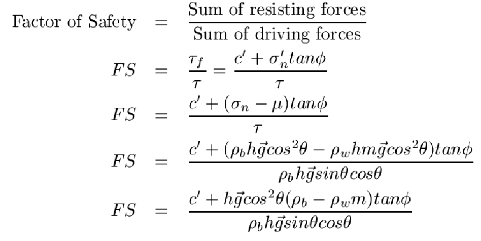
  FS = factor_of_safety(c_prime, h, theta, vr, rho_r, m, phi, v)

  This function calculates the factor of safety for an infinite slope
  stability problem.

  See Arrowsmith notes: http://arrowsmith362.asu.edu/Lectures/Lecture15/

  Author:
  JRA, 11/8/2006

  Variables:
         External
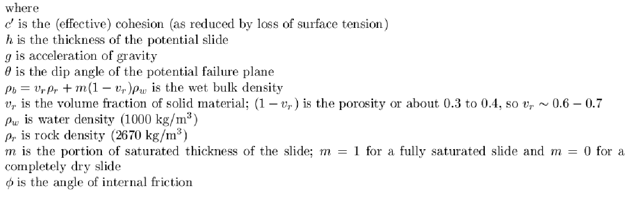
  c_prime is the (effective) cohesion (as reduced by loss of surface tension)
  h is the thickness of the potential slide
  theta is the dip angle of the potential failure plane
  rho_b = v_r rho_r + m(1-v_r)rho_w is the wet bulk density
  v_r is the volume fraction of solid material; (1-v_r) is the porosity
  or about 0.3 to 0.4, so v_r ~ 0.6-0.7
  rho_r is rock density (2670 kg/m^3)
  m is the portion of saturated thickness of the slide; m = 1 for a
  fully saturated slide and m = 0 for a completely dry slide
  phi is the angle of internal friction
  v stands for verbose. If v ==0, then supress output.

        Internal
  g is acceleration of gravity
  rho_w is water density (1000 kg/m^3)
  theta_rads is theta in radians
  phi_rads is phi in radians
  denominator = driving stresses
  numerator = resisting stresses

Here are some calculations to go with it:
This one is just past critical

>> factor_of_Safety(11900,   6,     10, 0.6, 2670, 1, 8, 1);
Constants
c = 11900.000, h = 6.000, theta = 10.000, rho_r = 2670.000, m = 1.000, phi = 8.000
Results
rho_b = 2002.000, FS = 0.989, theta = UNSAFE!

Slope goes up, safety goes down:

>> factor_of_Safety(11900,   6,     20, 0.6, 2670, 1, 8, 1);
Constants
c = 11900.000, h = 6.000, theta = 20.000, rho_r = 2670.000, m = 1.000, phi = 8.000
Results
rho_b = 2002.000, FS = 0.507, theta = UNSAFE!

Diminish saturation, safety goes up:

>> factor_of_Safety(11900,   6,     10, 0.6, 2670, 0.5, 8, 1);
Constants
c = 11900.000, h = 6.000, theta = 10.000, rho_r = 2670.000, m = 0.500, phi = 8.000
Results
rho_b = 1802.000, FS = 1.232, theta = SAFE!

Increase internal friction, safety goes up

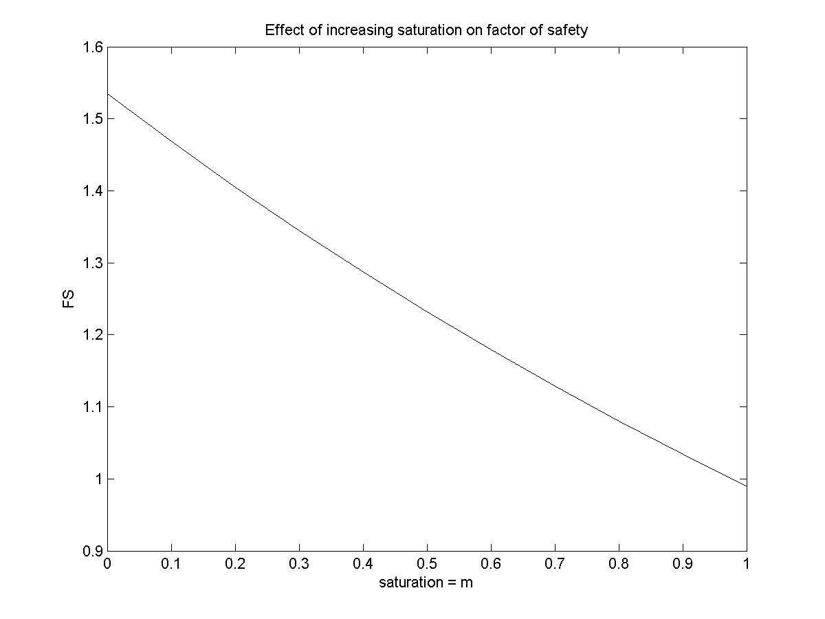
>> factor_of_Safety(11900,   6,     10, 0.6, 2670, 1, 16, 1);
Constants
c = 11900.000, h = 6.000, theta = 10.000, rho_r = 2670.000, m = 1.000, phi = 16.000
Results
rho_b = 2002.000, FS = 1.404, theta = SAFE!

Now how about a few plots:

m = 0:0.1:1;
fss = factor_of_Safety(11900,   6,     10, 0.6, 2670, m, 8, 0);
figure(1)
clf
plot(m,fss, 'k-')
title('Effect of increasing saturation on factor of safety')
xlabel('saturation = m')
ylabel('FS')
print('FSvsm.png', '-dpng')
>>

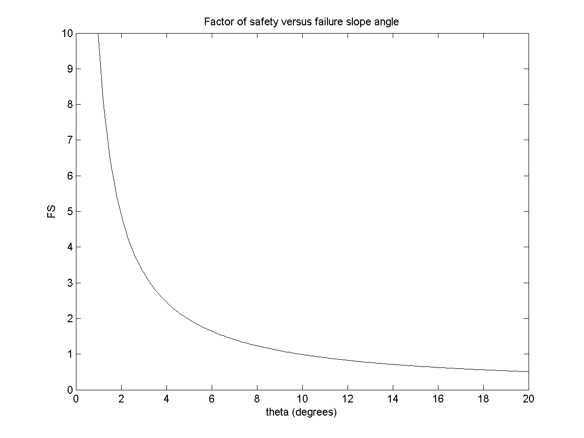
theta = 0:0.1:20;
fss = factor_of_Safety(11900,   6,     theta, 0.6, 2670, 1, 8, 0);
plot(theta,fss,'k-')
title('Factor of safety versus failure slope angle')
xlabel('theta (degrees)')
ylabel('FS')
axis([0 20 0 10])
print('FSvstheta.png', '-dpng')

GLG410/598--Computers in Earth and Space Exploration

Lecture 8: Programming in Matlab

Matlab scripts

Matlab functions

Example of a simple function:

More Control Flow: "If" Statements

Example Computation Using Functions: factor of safety