Gridding and Contouring Data

Graphics Handles

At this time, it is appropriate to introduce the concept of graphics handles. Graphics handles are values that are returned when calling some graphics functions which represent different aspects of the graphic that you are working on. For example, if I called the function

contour(myDistribution)

Matlab would return several numbers which act as references to the graphic that I just created with contour. These references are called ``handles'' and may be used to transfer the information created in the graphics function to another function. For example, when contour is called, handles are returned and may be put into the clabel function which will label the appropriate contour lines in the figure. An example of this is shown below.

Contour Plots

Matlab is capable of graphing three variables as a contour plot. In this system, there are two independent variables which are varied along the x- and y-axes with a resultant z-value. The z-values may be contoured as long as the function at any point does not have multiple solutions.

In order to demonstrate how to make a contour plot in Matlab, we will use some built-in Matlab functions to contour. For demonstration purposes, the function peaks is built into the Matlab system. In order to set a variable equal to this function, type:

Z = peaks;

This will fill the variable Z with the distribution and return a 49x49 matrix of values representing the Z-values of the distribution. If you wish to change the number of elements in the matrix, simply put those numbers in the parentheses in the peaks function.

There are several ways to contour data. First, you can make a basic contour plot in which the contour lines represent a given interval. Second, you can contour using area contours which color the area in between contours a solid color. A third variation on the contour plot is to have uneven contour intervals. This is especially useful when contouring data which may have a wide range of Z-values which may be logarithmically distributed, for example. We will start with the simplest case of making a plain contour plot and build into the more complicated scenarios.

To make a basic contour plot, we first need a distribution of data (a matrix of Z-values). This may have been created from some data that you have or we can call on Matlab's built in peaks function to create a matrix of Z-values for demonstration purposes. First, issue the command:

Z = peaks;

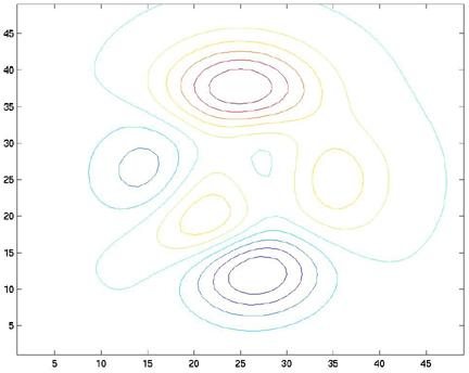
Next, you want to create a contour plot with ten contour lines and keep the reference handles of the contour plot in the variables c and h. To do this, issue the following command:

[c,h] = contour(Z,10);

Notice that the contour inverval of 10 is entered after the Z-value matrix. The result of this function is shown below:

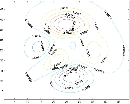
Now, let's put some labels on the contour lines. To do this, we will use the clabel command. The clabel command takes the contour plot's handles as arguments and will automatically label the lines:

clabel(c,h);

The result of this operation is:

title, xlabel, and ylabel commands, you can add annotation to your contour plot.

You can also interactively choose to label your contour lines using

clabel(c,h,'manual')

clabel(c,'manual')

This allows the user to place labels using the mouse.

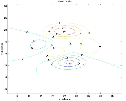
With contour, you can specify the size of each of the elements of the Z-matrix by passing contour two additional variables, a vector containing the X-values for each column in the Z-matrix, and a vector containing the Y-values for each row in the Z-matrix. For example, if the width of each of the elements in the Z-matrix is one and the height of each element in the Z-matrix is 0.5, you can make two vectors which let contour know this information. Use the incremental fill function (described above) to set the values of the X- and Y- vectors to their appropriate values:

X=1:49;
Y = 1:.5:25;
[c,h] = contour(X,Y,Z,10);
clabel(c,h);
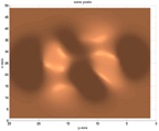
axis equal;
title('some peaks')
xlabel('x distance'), ylabel('y distance')

The axis equal command simply forces the size of the X-increment to equal the size of the Y-increment on the axes of the figure. If this is not done, Matlab will scale the axes to fit all of the data onto the plot.

Here is the plot:

The contour lines can also be defined by a vector. This is similar to the previous example, but we will define a vector, v.

v = [-5 -4 -3 -2 -1 0 1 2 3 4 5];
[c,h] = contour(X,Y,Z,v);		% <-- here we replace 10 with "v"
clabel(c,h);
axis equal;
title('some peaks')
xlabel('x distance'), ylabel('y distance')

Surface plots

Along with contouring, one can often make true 3D plots of datasets like the one above. You can do this with a couple of commands:

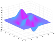
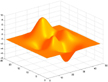
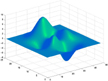
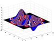
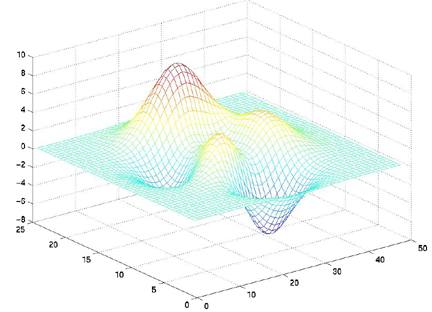
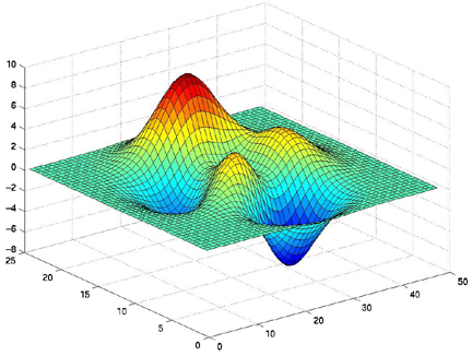
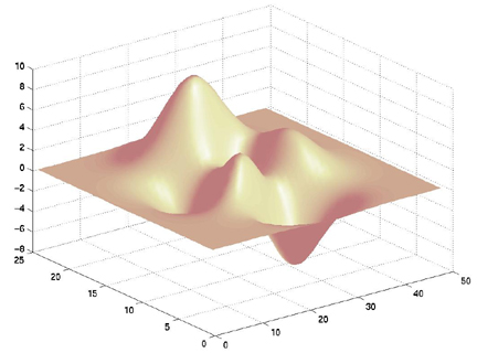
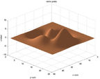
Z = peaks;
X=1:49;
Y = 1:.5:25;

mesh, surf, and surfl.

 mesh(X,Y,Z)

 surf(X,Y,Z)

surfl(X,Y,Z)
shading interp
colormap pink

Note that we have used the command shading interp with that plot. The shading function selects between faceted, flat, or interpolated shading. Although it can take more graphics computations, the interpolated shading usually looks best. We also used a colormap other than the default. The colormap is a data structure that is ues to represent color values. It is an array of three columns and some number of rows of RGB values. I have made the same plot as above with a number of different built-in Matlab colormaps:

colormap pink	colormap cool	colormap autumn	colormap winter	colormap flag	colormap copper

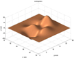
And here is the finally labeled plot with a couple of different versions of the view:

surfl(X,Y,Z)
shading interp
colormap copper
title('some peaks')
xlabel('x-axis'),ylabel('y-axis'),zlabel('z-label')
view(45,45)

view(45,45)	view(270,90)	view(135,35)

Gridding

In many cases in earth science, we do not have evenly spaced observations. We need to grid our unevenly spaced data by determining some set of evenly spaced estimates that approximate the observations. So let's take a simple dataset of topography from the Salt River bottom just north of ASU:
Here are the data.
You have to convert it into E, N, H vectors and get it onto the computer.
Then:

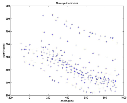
load('E.txt','-ascii');
load('N.txt','-ascii');
load('H.txt','-ascii');

First make a plot of E and N to see where they are located:

plot(E,N,'k+')

So you can see that they are irregularly spaced.
Now we will use the command griddata:

>> help griddata

 GRIDDATA Data gridding and surface fitting.
    ZI = GRIDDATA(X,Y,Z,XI,YI) fits a surface of the form Z = F(X,Y)
    to the data in the (usually) nonuniformly-spaced vectors (X,Y,Z)
    GRIDDATA interpolates this surface at the points specified by
    (XI,YI) to produce ZI.  The surface always goes through the data
    points.  XI and YI are usually a uniform grid (as produced by
    MESHGRID) and is where GRIDDATA gets its name.

    XI can be a row vector, in which case it specifies a matrix with
    constant columns. Similarly, YI can be a column vector and it
    specifies a matrix with constant rows.

    [XI,YI,ZI] = GRIDDATA(X,Y,Z,XI,YI) also returns the XI and YI
    formed this way (the results of [XI,YI] = MESHGRID(XI,YI)).

    [...] = GRIDDATA(...,'method') where 'method' is one of
        'linear'    - Triangle-based linear interpolation (default).
        'cubic'     - Triangle-based cubic interpolation.
        'nearest'   - Nearest neighbor interpolation.
        'v4'        - MATLAB 4 griddata method.
    defines the type of surface fit to the data. The 'cubic' and 'v4'
    methods produce smooth surfaces while 'linear' and 'nearest' have
    discontinuities in the first and zero-th derivative respectively.  All
    the methods except 'v4' are based on a Delaunay triangulation of the
    data.

    See also INTERP2, DELAUNAY, MESHGRID.

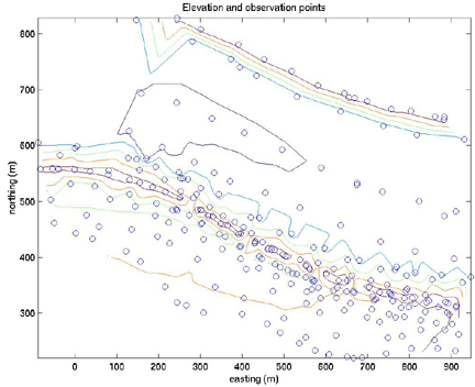
Basically, we need to tell griddata what the x and y grid looks like on which it will operate. So I did this for our topography:

>> estep = (min(E)-max(E))/100

estep =

  -10.3468

>> estep = abs(estep)

estep =

   10.3468


>> e = [min(E):estep:max(E)]

>> nstep = (min(N)-max(N))/100

nstep =

   -6.0886

>> nstep = abs(nstep)

nstep =

    6.0886

>> n = [min(N):nstep:max(N)]

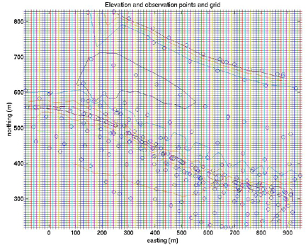
Those are the vectors of easting and northing positions for our grid.
Now, let's grid it:

[xi,yi,zi] = griddata(E,N,H,e,n');

Now, let's plot it:

contour(xi,yi,zi)
hold on
plot(E,N,'o')
xlabel('easting (m)')
ylabel('northing (m)')
title('Elevation and observation points')

plot(xi,yi,'+')
title('Elevation and observation points and grid')

Finally, let's look at it as a surface:

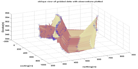
surfl(xi,yi,zi)
shading interp
colormap pink
hold on
plot3(E,N,H,'o')
title('oblique view of gridded data with observations plotted')
xlabel('easting(m)'),ylabel('northing(m)'),zlabel('Elevation(m)')
view (65,45)

More Examples