GLG410/598--Computers in Earth and Space Exploration


Announcements Syllabus Schedule Weekly lecture notes Assignments Links

Assignment 7: Gridding Irregularly Spaced Data in Matlab

In this assignment, you will be building functions for general gridding and contouring of data.

Matlab gridding and contouring functions

  1. Build a Matlab function to grid 3D data:
  2. Build separate functions to create each type of plot: (see this page for examples of these kinds of plots)
You will now use the functions you just built to work with two different datasets. These functions should be well adapted to work with many types of applications.

Topographic Data

Data: vmrrot2.txt

Topography is one of the most common types of data that needs to be gridded, contoured, and plotted in 3D for convenient visualization. You are given a text file that contains topographic data, where the columns are EASTING, NORTHING, and HEIGHT. This data is from an area of the San Andreas fault seen here.

TASK: Build a well-commented script that loads in this data and outputs the following plots: NOTE: Include the print command to save your plots as JPEGs
NOTE: Choose an appropriate contour interval size (it should look good, but fit the data)

Questions:

What are the landforms that you observe and how are they arranged?
Where would you put the San andreas fault (right lateral fault system)?
What is the evidence for offset along the fault zone?

Crustal Thickness and Bulk Composition

Data: ears_overview.txt

Continental crust is on average ~35 km thick and oceanic crust is ~7-8 km thick. However, there are large variations of this thickness around the globe. Seismology is often used to explore and map these variations within interesting tectonic regions. For this part of the homework, we will take a look at crustal thickness variations in our neck of the woods, southwestern US.

You are given a comma-delimited text file that contains data from the Earthscope Automated Receiver Survey (EARS). This study by several researchers at the University of South Carolina uses seismic data recorded by the USArray component of the Earthscope project to perform automated processing using the receiver function technique. The term receiver function just refers to a waveform that represents the velocity structure of the Earth directly below a given seismic station. This processing method uses different components of motion at individual seismic stations to look for waves that are refracted and converted at the base of the crust. This technique has been used effectively to map the thickness of the crust and get estimates of the P/S wavespeed ratio (Vp/Vs). The Vp/Vs ratio can be used to compute Poisson's ratio, which has implications for bulk crustal composition. In general, lower Vp/Vs is indicative of felsic composition, whereas higher Vp/Vs is indicative of mafic composition.

Dealing with text formats

This will be a good lesson on dealing with different formats of text files. Not everything that you deal with is easily loaded into Matlab using the load function.

Columns in "ears_overview.txt":
Network Code, Station Code, Station Latitude, Station Longitude, Station Elevation, Crustal Thickness, Std. Dev. (thickness), Vp/Vs, Std. Dev. (Vp/Vs), Assumed Vp, Vs, Poissons Ratio, Number of Earthquakes Used, Residual Complexity

Here is a function you can use to import the comma-delimited data into Matlab (ImportCSV). For the columns that you want to use as numeric data, try this command to convert the cell array to a numeric array:
for n = 1:length(Column08)
    if isempty(Column08{n})
        NewColumn08(n) = NaN;
    else
        NewColumn08(n) = str2num(Column08{n});
    end
end
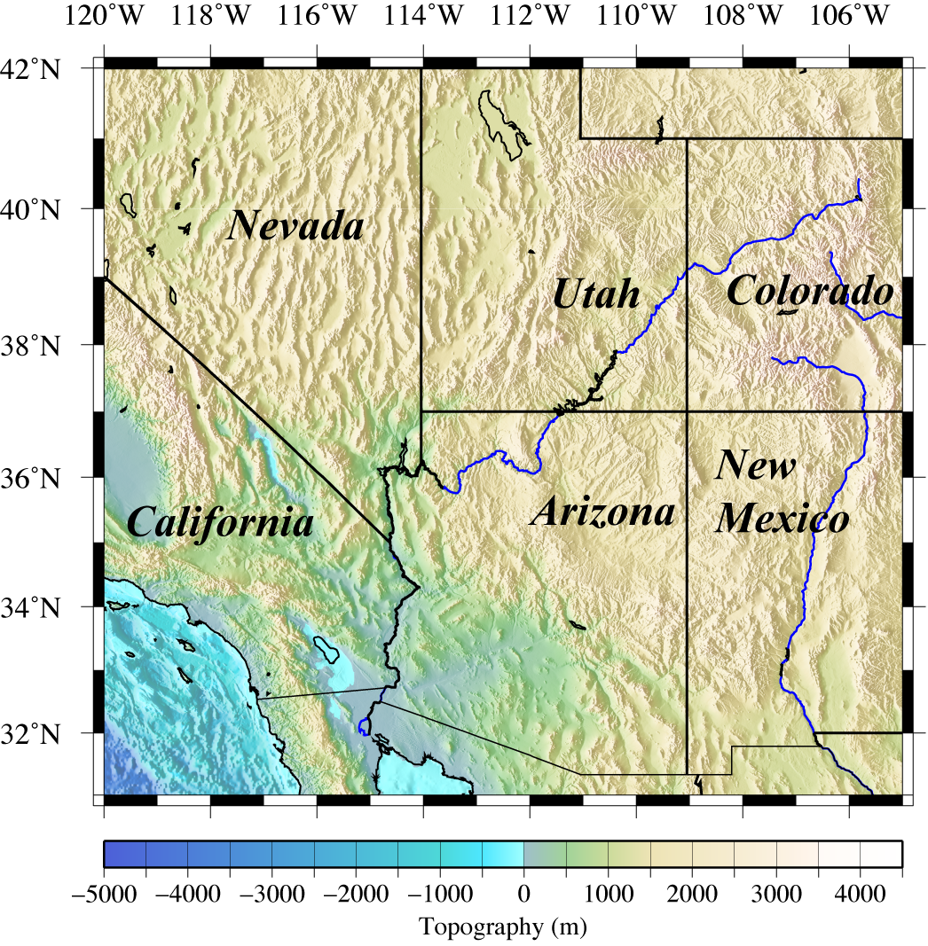
You will need to subset this data because this file includes global data. Only include stations between longitudes -120 and -105 and latitudes 31 and 42. You know how to do this from previous homeworks.
Let us concentrate on the crustal thickness and Vp/Vs of the southwest US.


TASK: Build another well-commented script that loads in this data and outputs the following plots: NOTE: Include the print command to save your plots as JPEGs
NOTE: Choose an appropriate contour interval size (it should look good, but fit the data)

Questions:

Are there obvious regions of thick or thin crust?
Is there a correlation between crustal thickness and topography? Refer to the map of topography below.
Are there an areas with obvious changes in Vp/Vs?


Website

TASK: Include the follow:

Grading Rubric (50 poionts)

Assignment is due Monday, March 16, 2009.

GLG410/598 Computers in Earth and Space Exploration


Last modified: March 5, 2009