Digital Elevation Models and Simple Maps in ArcMap
In today's lecture we will learn how to:
Acquire NED and DOQ data from the USGS seamless data warehouse. NED stands for
National Elevation Dataset, which provides
nation-wide coverage of a digital elevation model (DEM). DOQ stands for
Digital Orthophoto
Quadrangle and is basically a georeferenced and rectified aerial photograph.
Load these datasets into ArcMap and project them into the correct coordinate
system.
Produce a hillshade from the DEM.
Produce a simple map in ArcMap.
(1) Acquire NED and DOQ data from the USGS seamless data warehouse
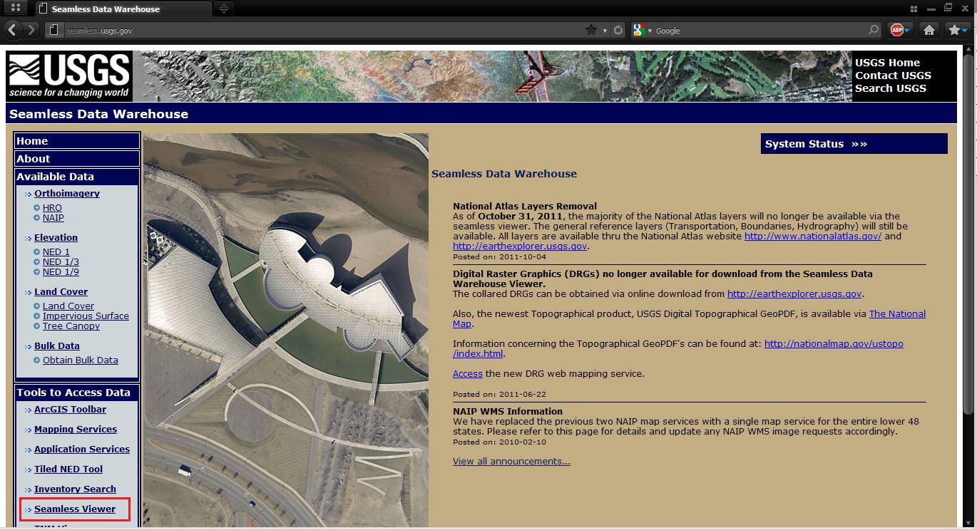
The USGS provides the following web access from which a variety of geospatial
data may be downloaded: http://seamless.usgs.gov.
On the left side of the page under Tools to Access Data, click Seamless Viewer.
This will take you to the National Map Seamless Server interface from which we will
download our elevation and imagery data.
This site tends to be sluggish, so try to be patient when doing things like zooming, panning,
and downloading data.
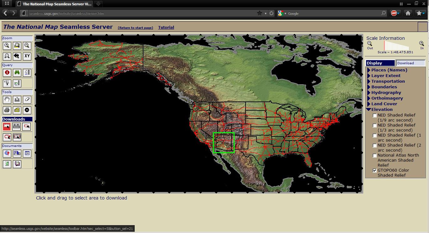
The left panel contains tools for navigation and downloading. The central panel is the
data viewer. The right panel is the Display and Download options. The Display
tab lets you choose the data you want displayed in the viewer. The Download tab
lets you choose the data you want to download to your computer. Each tab has several data
options from which to choose (e.g., Transportation, Elevation, Orthoimagery). Right now
you will notice that under the Display tab the "GTOPO60 Color Shaded Relief" box is checked,
which is thus displayed in the main viewer.
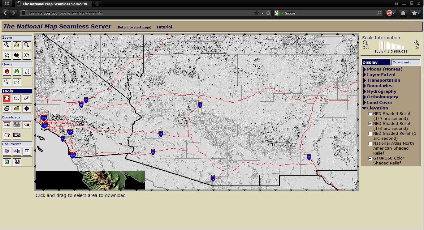
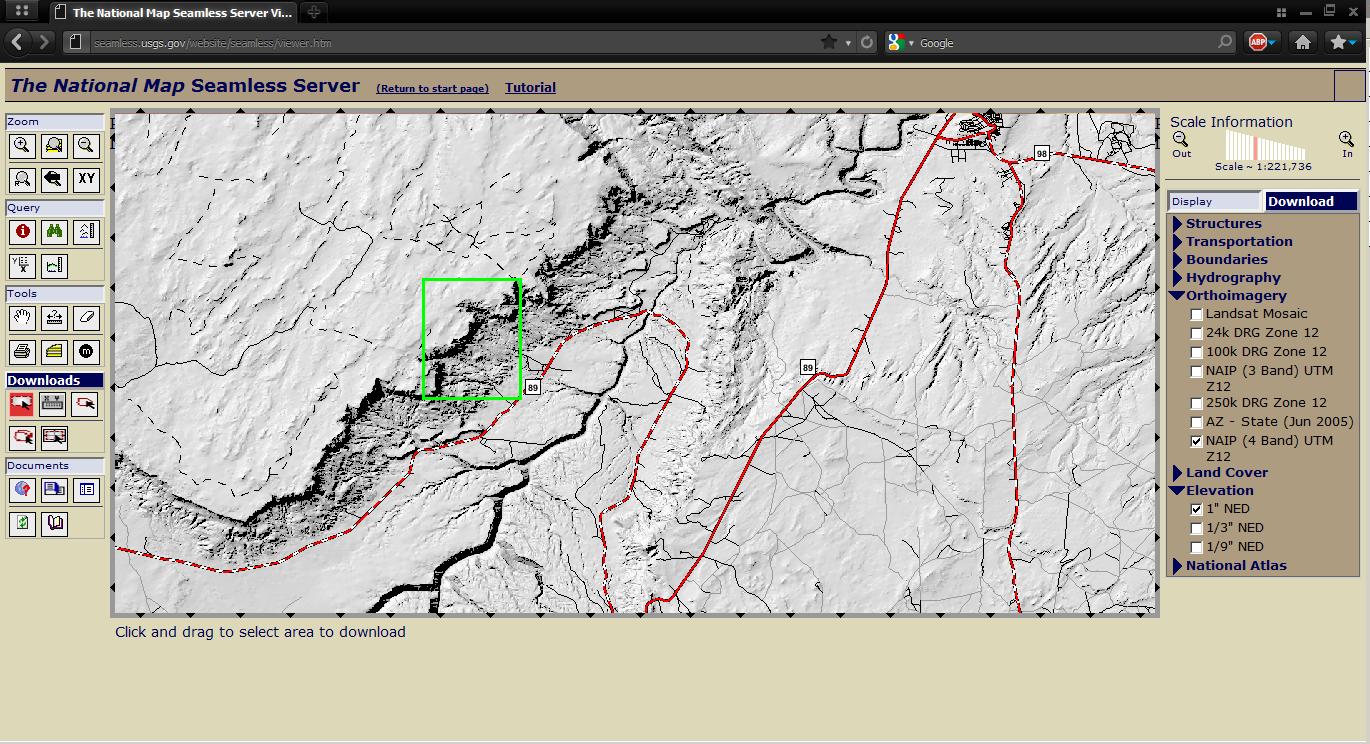
Zoom into any area of interest. Here I chose to zoom into part of the Vermilion Cliffs
near Marble Canyon, AZ. One thing to note is that depending on which area you zoom into,
there will be varying availability of datasets. For our example, we can see that there
are several elevation and orthoimagery datasets that I can download for the Vermilion Cliffs.
Under the Download tab, expand the Orthoimagery and Elevation menus to see what data are
available. Select the NAIP (4 Band) UTM Z12 box from the Orthoimagery menu and the 1/3"
NED box from the Elevation menu.
IMPORTANT: Before proceeding to the next step, disable any pop-up blockers that may
be configured in your browser.
Select the region of interest using the download tool in the left panel.
The following window will pop up listing the available downloadable datasets for your
area of interest. Click the datasets you wish to download to your computer. This will
open up several other windows (e.g., extracting data, downloading data) and may take
several minutes to complete the download depending on the size of your area of interest
and the resolution of the data you requested.
Your data will be downloaded as zipped files. Unzip the data into two separate folders
named "NED" and "DOQ".
IMPORTANT: if you are working on your laptop, create a new folder called "GIS" and
place these datasets in there. If you are using MyApps, create a new folder in your M drive
called "GIS" and upload these datasets to that directory. This is greatly facilitated by
using a Secure File Transfer client (SSH for Windows or Fetch for Mac) instead of MyFiles.
Review how to do this on our
Create your website page.
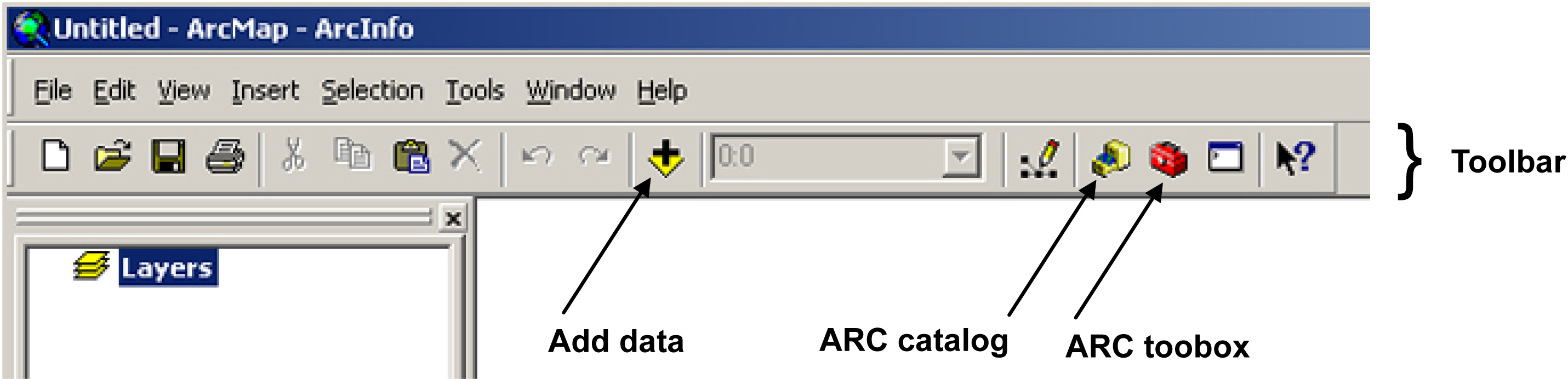
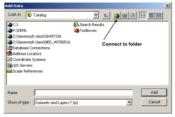
Start ArcMap and click the Add Data button. This will open up a window that will let us browse to
the data. Click the Connect to folder button and navigate to the directory that
contains your data. Click OK. This will add that directory to the Add Data window. Navigate
to your NED data folder in your GIS directory, select the DEM file (extension .tif), and add it.
Behold the Vermilion Cliffs DEM!!
Now is a good time to save your ArcMap project (as a .mxd file) somewhere in your GIS directory.
Project the DEM in ArcMap
Notice that the map units are in decimal degrees (located near the bottom-right corner
of the ArcMap window). It's much easier to think in meters than decimal degrees, so we're
going to project the DEM into the
UTM coordinate system. But before we do this, let's first check in which UTM zone the
Vermilion Cliffs are located. Using the UTM
Grid Zones of the World webpage compiled by Alan Morton, we see that the Vermilion
Cliffs are located in UTM Zone 12. In fact, almost all of Arizona is located in UTM Zone 12!
In ArcMap, start ArcToolbox (little red toolbox icon) and navigate to Data Management
Tools --> Projections and Transformations --> Raster --> Project Raster (double click).
Click and drag the DEM layer from the Table of Contents to the
Input Raster field. You will notice that this automatically fills in the Input
Coordinate System field for you, in our case telling us that our DEM is in the
GCS_North_American_1983 coordinate system. For the Output Raster Dataset
field, click the browse button and navigate to the directory to which you want ArcMap to
write the new projected DEM. Give the projected raster a new name. For the Output
Coordinte System field, click the browse button and make sure you are in the
XY Coordinate System tab. Click the Select button and navigate through
Projected Coordinate Systems --> UTM --> NAD 1983 UTM Zone 12N (double click). Then,
in the Resampling Technique (optional) field, select CUBIC and hit OK. This
will begin the projection process and may take a minute or two depending on the size of
your DEM.
Once the newly projected DEM is displayed in ArcMap, go ahead and remove the old unprojected
DEM layer from the project (right click and select Remove).
Now is a good time to save your project (Ctrl+S or hit the save button).
Note that ArcMap defines the projection of the entire project according to
that of the layer that was first added. So for our example, our ArcMap project is still in
the old projection! To fix this, go to the Table of Contents panel, right click
Layers and click Properties. This will open up the Data Frame Properties window.
Under the Coordinate System tab navigate through Predefined --> Projected
Coordinate Systems --> UTM --> NAD 1983. Select NAD 1983 UTM Zone 12N and click OK.
This will change the projected coordinate system of the entire project.
But notice that the map's units are still in decimal degrees even though our data are in
meters. To change this, open the Layers properties again (right-click --> Properties), click
the General tab, change the Display units to meters, and click OK. Now the map units
are displayed in UTM meters.
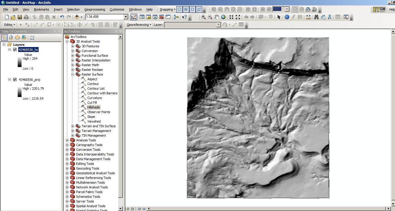
(3) Produce a hillshade from the DEM.
You might have noticed that our DEM doesn't really show much beyond what looks like a
simple drainage network. To improve the visualization of these data, we will build an
artificially illuminated hillshade from the DEM.
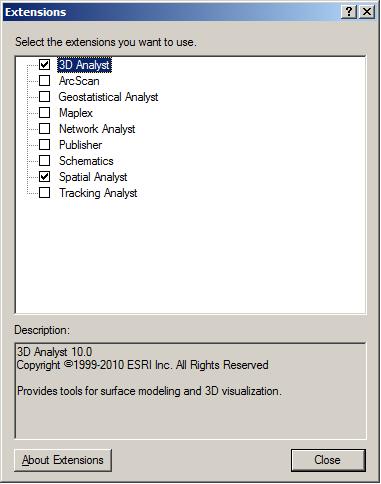
Before we do this, we first need to enable the 3D Analyst and Spatial Analyst
extensions in ArcMap. In the main ArcMap toolbar, go to Customize --> Extensions...
and check the 3D Analyst and Spatial Analyst boxes.
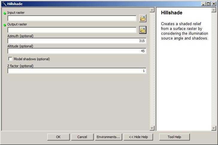
In ArcToolbox, minimize any expanded tools you have open and navigate through 3D Analyst
Tools --> Raster Surface --> Hillshade (double click).
Click and drag the newly projected DEM to the Input raster field.
In the Output raster field, browse to the directory in which you want ArcMap to create
the hillshade. Hit OK and the hillshade processing should begin:
Now is a good time to save your project.
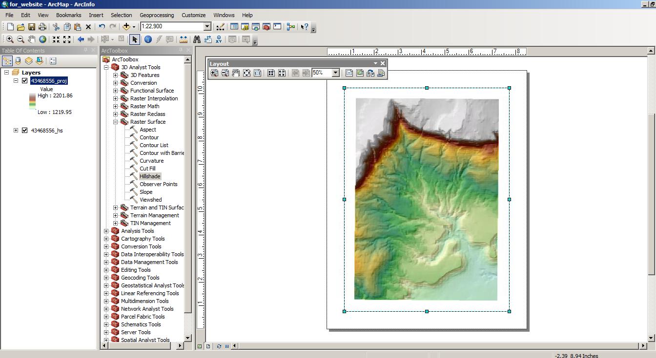
(4) Produce a simple map in ArcMap.
Let's turn our ArcMap project into a nice map. In the Table of Contents panel,
click and drag the DEM layer above the hillshade layer. We are basically rearranging
the layers so that the DEM layer is displayed above the hillshade layer. Now change the color of
the DEM layer by clicking once on the DEM's color ramp and selecting a color ramp of your choice.
Right click the DEM layer and select Properties. This will open up this layer's properties
from which we can change many things associated with this layer. Select the Display tab and
change the Transparency field to 40%, then hit OK.
Let's add some important components to our map: a scale bar, north arrow, and a vertical scale. Near
the bottom of the map panel is the Layout View button. Clicking it will take you to the layout
view of your map. This is basically what our map would look like if we were to print it.
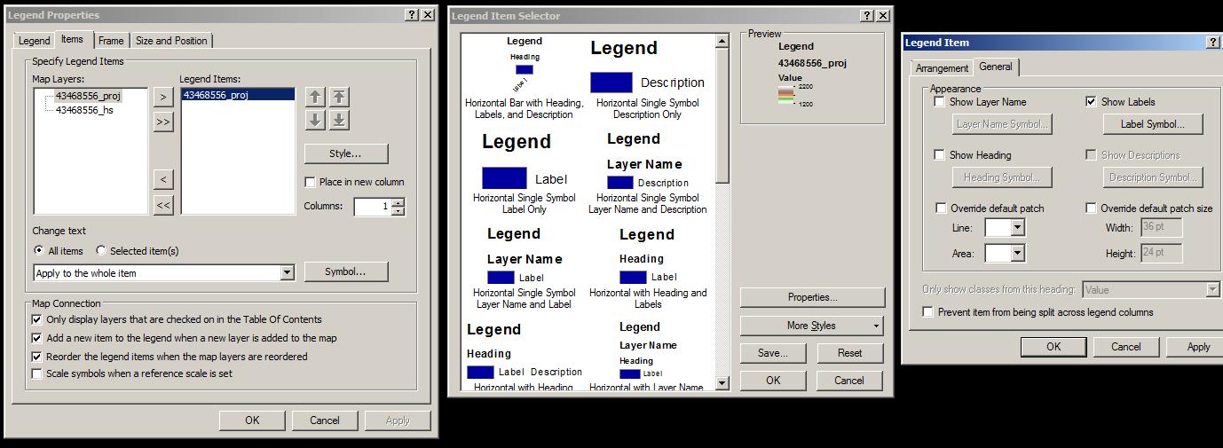
In the main ArcMap toolbar, click Insert -- > Legend . You can toggle which layers to include
in the map's legend by using the left- and right-pointing arrows. For our map, let's just include the
DEM layer in our legend.
Our legend looks OK, but Tufte would definitely not be happy with us considering the unnecessary
information present there. For example, let's get rid of all those significant digits and round up/down
the elevation extents for our map. To do this, right click the DEM layer in the Table of Contents
panel and select Symbology. In the Label fields, delete the "High:" and "Low:" text and
round the elevations to whole numbers. Click OK.
We still have unnecessary information like the layer's name. Right click on the legend itself
and select Properties. Click the Items tab, then the Style... button, then the
Properties button, and finally the General tab. Unselect the Show Layer Name and the
Show Heading boxes.
OK out of everything to return to the map.
Now that's not a bad-looking map! :-) But it still needs a scale bar and a north arrow. These can be added
using the Insert menu from the main ArcMap toolbar. Experiment with these to make your map look
reader-friendly. Mine looks like this:
Don't forget to save your project!
Some video demos of ArcMap routines using LiDAR topography as an example
The following videos are demonstrations for some useful activities in ArcMap. Check them out and
practice!
Load and fix a standard DEM (no info file) into ArcMap 10:
Mosaic standard DEMs into new raster in ArcMap:
Combine color gradient of topography for elevation with the hillshade to make a nice map for visualization:
Make a simple map layout, explanation, and export to PDF:
Make a slope map and a slopeshade in ArcMap:
Compute and display contours in ArcMap:
Point and Profile queries:
Page written by David Haddad and Ramón Arrowsmith, with some items borrowed from
Olaf Zielke.
Last update: October 21, 2011.