GLG410/598--Computers in Earth and Space Exploration


Announcements Syllabus Schedule Weekly lecture notes Assignments Links

3D image visualization in ArcScene

It is sometimes useful to visualize imagery such as digital orthographic quadrangles (DOQs) in 3D using elevation data from digital elevation models (DEMs). The ArcGIS suite has a simple program called ArcScene designed to do just this and operates very much like ArcMap.
Let's do this using last lecture's datasets:
Projected Digital elevation model (DEM)
Digital orthophoto quadrangle (DOQ)

Load the DEM in ArcMap

Start ArcScene and click the Add Data button. This will open up a window that will let us browse to the data. Click the Connect to folder button and navigate to the directory that contains your DEM and DOQ data files. Click OK. This will add that directory to the Add Data window. Navigate to your NED data folder in your GIS directory, select the DEM file (extension .tif), and add it.

This is a perspective view of the DEM. Notice that it doesn't have any topography. Recall that for each of the DEM's (x,y) pixels there is a z value for elevation. So we need to somehow "drape" each pixel over its elevation value.
Right click the DEM layer under Scene layers and select Properties. Click the Base Heights tab.


Select the Floating on a custom surface radio button and browse to the directory that contains the projected DEM. It is imported to use the projected DEM for this step!
Select the DEM file and click Add. Notice that we also have the option to change the vertical exaggeration of our 3D scene by changing the Factor to convert layer elevation values to scene units value. For now, let's use the default value of 1 and not vertically exaggerate the topography. Hit OK.


Now is a good time to save your ArcScene project (as a .sxd file) somewhere in your GIS directory.

This looks good for the DEM. How about doing the same thing for the DOQ image? First, remove the DEM layer from the project, then add the DOQ layer using the Add button. Repeat the steps of adding base heights to the DOQ as we did before.


Now that's a nice looking 3D image of the Vermilion Cliffs!

Experiment with the Tools toolbar to see how the navigation and fly-through controls work.


Don't forget to save your project!

Assignment 9: Digital Elevation Models and the USGS' seamless site

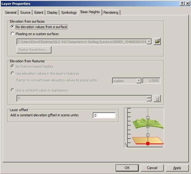
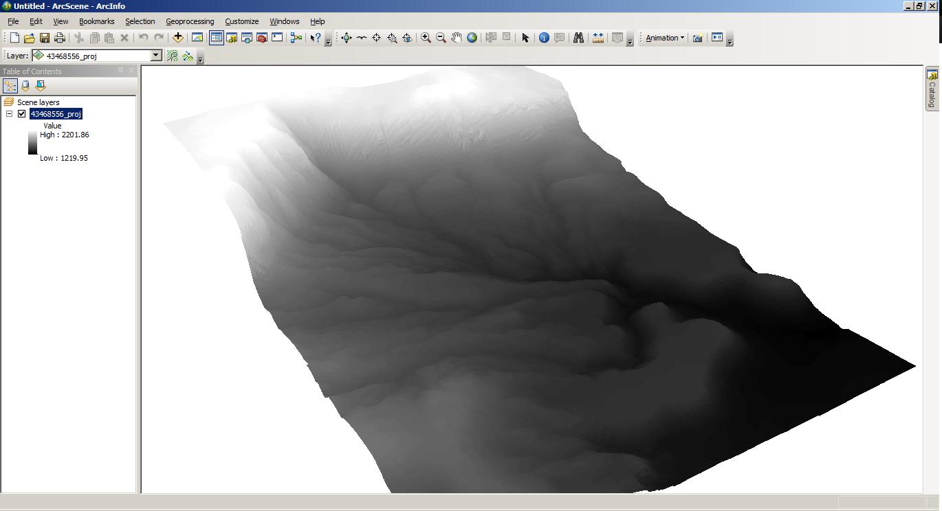
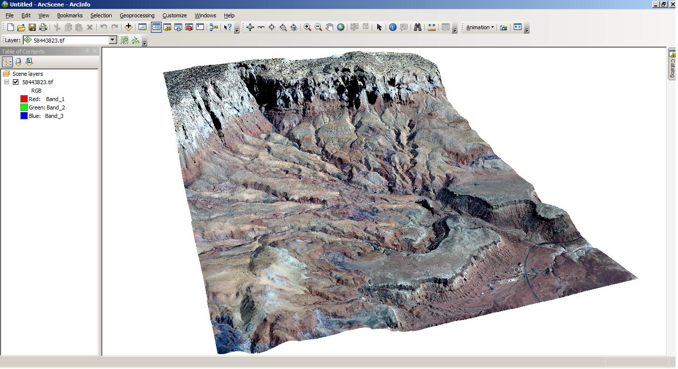
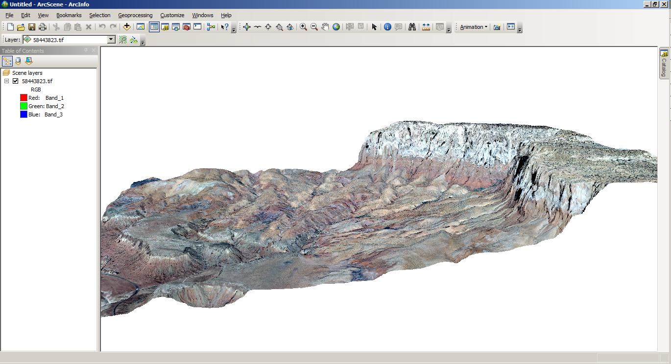
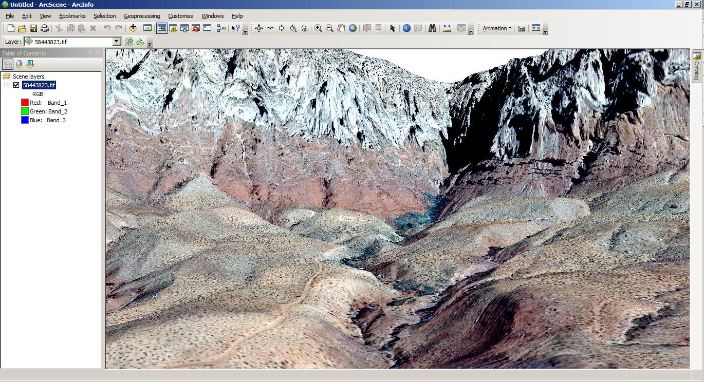
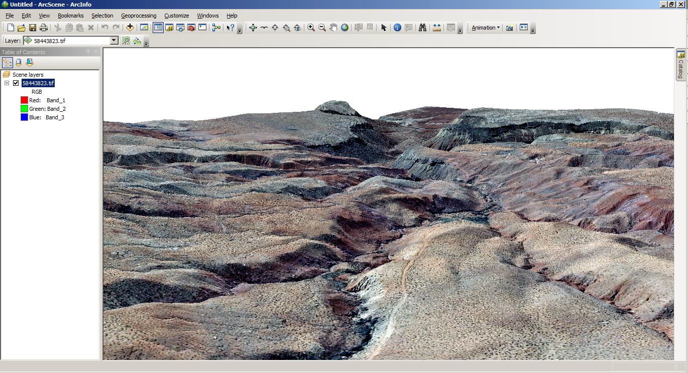
This assignment is designed to help you learn the tasks that we described in the last two lectures on Digital Elevation Models and Simple Maps in ArcMap and Enhanced imagery visualization in ArcScene.

Main tasks:

I. For any place in the US with Seamless coverage, choose a landscape or landform of interest (but be careful not to choose too large of an area, or ArcGIS and Seamless won't be happy) and follow the demonstration from the DEMs in ArcGIS lecture and produce the following items:
  1. A nice map with color-coded and semi-transparent elevation and hillshade. Make sure to add an explanation and scale bar. Post the map to your web site as an image. In addition, write a one paragraph description of the landscape depicted in your map and post your answer below the map on your website. Try to stick to basic description, don't do other research. Emphasize only what you can see in your map. Here's an example from the South Mountains:
    "This view of the eastern South Mountains near Phoenix Arizona shows a NE-trending mountain rising to about 780 m (about 450 m above the adjacent basin). The range is cut by valleys trending mostly parallel and some normal to the ridge axis. The transition between the mountain front and the basin is intricate and sinuous. A satellite range with an axis parallel to the main range is evident in the southwest. To the northeast, several small hills decorate the basin floor. The hills and the intricate range front are consistent with sedimentation and burial of the foot of this range and indicate its likely prior greater extent."

II. For a different place in the US, choose a landform of interest in Seamless (different from the one above, but be careful not to choose too large of an area, or ArcGIS and Seamless won't be happy) and follow the demonstration from Enhanced imagery visualization in ArcScene to produce the following:
  1. A 3D view of the topography with at least two different and interesting views of the feature. Export the image as a .pdf and post it to your website.
  2. A 3D view of the area depicted in some imagery (see what is available under the orthoimagery Download tab once you have found your target of interest from Seamless), with at least two different interesting views. Export the two views as .pdf files and post them to your website.
  3. Write a one paragraph description of the landscape depicted in your views and post your answer below the map on your website. Try to stick to basic description, don't do other research. Emphasize only what you can see in your 3D views, including what you see in the actual imagery. Here's another example for the South Mountains:
    "This view of the eastern South Mountains near Phoenix Arizona shows a NE-trending mountain rising to about 780 m (about 450 m above the adjacent basin). The small drainages trend opposite to the view. The range is irregular due to the incision of the drainages while the basin is rather flat in the foreground. Between the two, the piedmont steepens as it approaches the range, contacting it in a sharp and sinuous boundary between aggraded sediments and the bedrock of the range. The DOQQ imagery clearly shows the contrast between the finely textured urban area adjacent to the undeveloped (but trail covered--white sinuous lines) mountains. The boundary between the urban environment and the range is abrupt. The foreground shows larger patches of land associated with light industry."

Grading Rubric (50 points)

Assignment is due Thursday November 3, 2011.


Page written by David Haddad with some items borrowed from Olaf Zielke.
Last update: October 27, 2011.