Lecture 6: Curve fitting and the Solver using Excel
A note on being computing scientists and homework
So far, the Excel assignments have been with a fair bit of guidance, even with step by step recipes. However, you now have enough tools under your belt to tackle problems with out the step by step instructions. As the semester carries on, you will be doing more and more of the work with out such detailed instructions. I will try to provide some more tutorials, but I am expecting that you are reading the assignments and asking questions in class when we do the demos!
Today, we will experiment with curve fitting using Excel. First, we'll explore Excel's built-in "Trend-line" option, where we can add trend lines to data sets after a chart has been generated. Later, we will utilize an Excel tool called Solver, whereby we can fit a data set to more general functional forms, i.e., more freedom than a straight line, exponential, logarithmic, etc.
Curve fitting using the Add Trendline option when right clicking a data series point in a chart
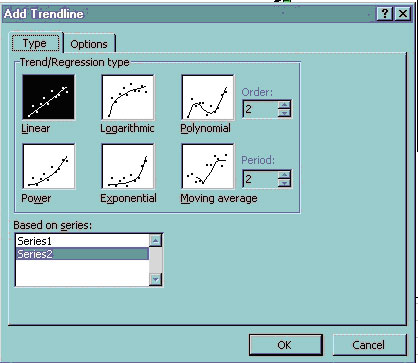
All you have to do is to right-click a data point within a chart then select Add TrendLine. There are many options:
Let's quickly discuss this with the following spreadsheet: (download this from the web to your disk space):
L05_climate.xls (Mean Tempurature perturbations for the US (in degree Celsius). Perturbation is the difference from the beginning of 1900 in this case.)
Try the linear fit. Do you think it is getting warmer? How hot will the average be in 2050? (You have to calculate this. Hint: show the equation by right-clicking the trendline itself and select Format trendline. Look for Display equation on chart. Try the ten year moving average--what do you think now about your linear projection?
If you are to be your own computing scientist, you should look into what Excel is assuming. The equations behind these options can be found from Excel's Help page:
For R2, it is based on two sums of squares: Sum of Squares Total (SST) and Sum of Squares Error (SSE). SST measures how far the data are from the mean and SSE measures how far the data are from the model's predicted values. The closer R2 is to 1, the better the fit. We will talk about least squares later in the lecture.
Curve fitting using Excel's SOLVER function
If we did not want to use an equation of a line to fit to data, or any of Excel's other options -- no problem, we can use Solver to do this. To simply fit a line to some data, the Trendline function is easiest. If we wanted to fit data to some specific function not contained in Excel's Trendline options, then we'd try Solver. Solver basically will help us find solutions that best satisfy inputted constraints. Let's look at a simple example. Download the following file from the web to your disk space:
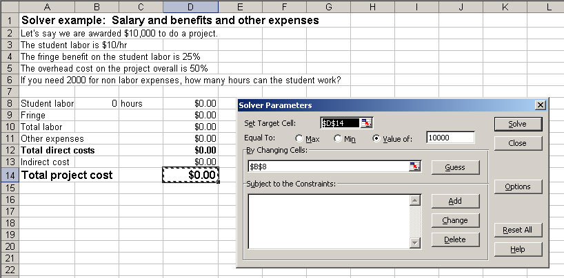
This example is a simple budgeting problem that I seem to have all the time.
First, you will need to add the Solver function to your tool belt if you haven't yet:
OLDER EXCEL: do this with the Tools>Add Ins menu. Check the Solver box. Once Solver is added, go to the Data>Solver... option to open Solver.
Office 2007:
Click the Microsoft Office File menu, and then click Excel Options.
Click Add-Ins, and then in the Manage box, select Excel Add-ins.
Click Go.
In the Add-Ins available box, select the Solver Add-in check box, and then click OK.
Tip:ĀIf Solver Add-in is not listed in the Add-Ins available box, click Browse to locate the add-in.
If you get prompted that the Solver Add-in is not currently installed on your computer, click Yes to install it.
After you load the Solver Add-in, the Solver command is available in the Analysis group on the Data tab.
While this is perhaps a silly example, it makes a couple points. For one, you can see our functional form is not of the type
y = mx + b.
Thus, we can't use the Add Trendline function to optimize a fit to our equation. We want to minimize the target cell E4 (the total cost), so make sure the Min radio button is selected. Then click Solve.
Curve fitting and Least Squares
Instead of finding a minimum of a functional form, we will find the minimum of the RMS which stands for root mean square.
where p is the number of observations, Hi is the observed value at xi, and Hmodel(xi) is the model (or calculated value) at xi. Thus, if we can minimize this measure, the root of the square of the differences between model (prediction) and observation, then we will be getting a best fit according to our description of "goodness" of fit.
Today, we will use Solver to obtain a best fit to a data set of ocean floor sedimentation rates. Let's work with these data of age of sediment versus depth below the seafloor:
Depth (cm)
Sedimentation Age (years)
407
10510
545
11160
825
11730
1158
12410
1454
12585
2060
13445
2263
14685
Can we figure out the sedimentation rate from these data? Yes, if we assume a functional form (e.g., linear, quadratic, etc). For sedimentation, let's assume the sedimentation rate stays constant, thus the equation should be linear, i.e., of the form y=mx + b. To analyze these data, we will solve this problem two ways:
(1) Use Add trendline on a chart made from these sedimentation data
(2) Use Solver to do the same thing.
This will show you another approach for determining best fit models to data sets. Open a new Excel workbook, and we will put each approach on a different sheet
Automatic way: Add trendline
Copy the above data into Excel. Make a chart of the data (XY scatter plot). Fit the data with a straight line, using Excel's built-in Add Trendline function. Choose the Linear option. Also, click the "Options" tab and choose to display the equation on the chart. Here is a picture of what that might look like (you'll notice that I changed the Y-axis range so that the data span is more appropriately represented in this dimension - always de-junk your chart!):
There, that was easy. If you're just fitting a line (or one of the other automated functional forms), this is really the way to do it. Done.
Less automated, but more flexibility: Solver
To illustrate the concept of Solver, we'll solve the same problem by finding the m and b that minimizes the RMS (root mean square - a measure of the misfit of the model to the data). To do so, follow these instructions:
Somewhere on a clean worksheet (e.g., below your freshly copied data table), define two cells, one for slope "m" and another for the Y-intercept "b". Go ahead and stick some number in each (they'll get updated later) and define names for those cells: I recommend naming them m and b. Also, put your estimates in the sheet next to each other (view my spreadsheet in the next image in these notes).
Set up a column of model age estimations that uses our guess of m ands b, call this Y_calc which equals m*x + b, where the x values are the depths of the observations, and m and b are our model parameters that describe our best fitting line (see Column C in image below).
Determine the RMS between the observed and modeled values: make a column that calculates the difference between the observed ages (Y_obs) and those you just estimated from your guessed m and b (Y_calc) [my column D in image below]. Note that these differences are called the residuals. In a column to the right of this (Column E), square that difference.
Calculate the sum of those squares (thus, simply sum the values in column E), then take the square root of this number, then finally divide by the number of observations. NOTE: count the number of observations using Excel's function count(cell range). If your data set had 100's or 1000's of data, you'd surely do it this way. This is the RMS, and what we will minimize using Solver. Make sure you understand what we're doing: we are computing the misfit of each data point to your line, and then squaring this. Then... we sum these up, square root, divide by the number of observations. Thus, this is essentially a weighted average of our misfits of our model (i.e., the RMS). Hence, minimizing the RMS will minimize our model's misfit. Understand this.
Your sheet might look like this:
Finally, open Solver under the Tools menu, and set it up to make the target cell the one containing your estimation of the RMS (F9 in my sheet) a minimum (click the Min button) by varying the cells that contain m and b (the cell range that is dashed below). It might look like:
Click Solve, Then you will find that after the solver finishes searching for the best fit, it will ask you if you want to keep the result, which of course you do. It will also offer a report (usually on a separate worksheet), select the Answer sheet option.
Finally: compare your answers for the best m and b values (i.e., the ones Solver obtained) to those calculated by the Add trendline function.
Bonus: Use your final fitted equation to extrapolate to determine what age the sediments should be at 5000 cm, assuming the constant sedimentation rate.
In the file DEWIJS.txt are a number of measurements of the percentage by volume of Zinc in rock samples from a mine area. The data come from 118 assays in 2 meter increments along a sphalerite-quartz vein. The data are ordered along the vein.
Import the data into your spreadsheet.
Make a plot of the Zn content along the vein
Study the data and compute the following: Min, Max, Mean, Mode, Median, Standard Deviation, Relative Standard Deviation.
Plot the data in a Frequency histogram. Using the drawing tools in your spreadsheet, label the Mean and Standard deviation.
Use those evaluations to describe the Zinc deposit and its potential in a few sentences narrative to a prospective buyer of the deposit.
After some mapping of the area, you determine that about 500 cubic meters of the vein can be economically mined. Using your mean and the standard deviation, determine the approximate range of likely cubic meters of Zn that will be recovered.
Upon further discussion with the financial people in your company, the estimation of how much can be extracted gets trickier:
Zn is valued at about $5,000 per cubic meter
The cost to mine it is $1,000,000 for the first 500 cubic meters.
Then, the cost goes up by each additional cubic meter exponentially. So the equation for the cost is 1,000,000+(amount mined > 500 cubic meters)2.
In your spreadsheet, make a column of volume mined (go from 0 to about 7000 m3 in steps of 500 m3). To the right, make a column of Cost to mine. In the third column, compute the value of the Zinc mined. Finally, in the fourth column, compute the difference between the cost and the value.
Plot both the cost and the value on the same chart. Where do the lines cross? That is the break even point.
Using the equations you set up for the cost to mine, the value, and the difference, use the solver to figure out exactly what the break even about is. Hint: Set the difference between the cost to mine and the value to 0 by changing the volume mined. Note that sometimes Excel will not get exactly to zero, but will be at something like 10-7 which is close enough.
If your company wants a decent profit (like $5,000,000), what should the amount mined be?
This assignment is due by the beginning of class, September 23 as a link on your assignments web page. Make sure that your spreadsheet is well organized, formatted, and annotated.
Video explanation of the assignment and tour of completed spreadsheet