Simple looping and matrix construction in Matlab

Introduction

This lecture is our fist introduction to what is called "control flow" in programming. We will start out with For Loops to demonstrate how you can do many repetative tasks without explicitly writing each successive iteration.

For loops

Help on for loops can be found here.
Sometimes, you need go go through a data set to do some analysis and you cannot do it in the simple vector mode of Matlab. For example,

>> for n = 1:5
n
end

n =

     1


n =

     2


n =

     3


n =

     4


n =

     5

Set up the example

Let's go back to our Yellowstone seismicity data.

I am going to load the data, set up a few variables, and then plot it:

load('ystone_eqs_sort.txt','-ascii');
year = ystone_eqs_sort(:,1);
x_locations = ystone_eqs_sort(:,4);
y_locations = ystone_eqs_sort(:,3);
depth = ystone_eqs_sort(:,5);
magnitudes = ystone_eqs_sort(:,6);

figure(1)
clf
plot(x_locations,y_locations,'k.')
xlabel('longitude')
ylabel('latitude')
axis equal
hold on

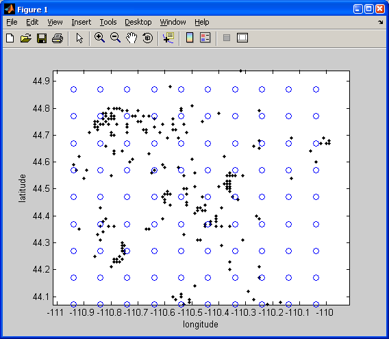
One loop

stepsize = 0.1;
long_range=min(x_locations):stepsize:max(x_locations);
for long = long_range
   plot(long,min(y_locations),'bo')
end

Here we need to specify the step size as we move across the grid. Notice the blue circles across the base:

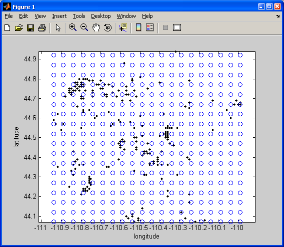
Nested loops

stepsize = 0.1;
long_range=min(x_locations):stepsize:max(x_locations);
lat_range = min(y_locations):stepsize:max(y_locations);
for long = long_range
    for lat = lat_range
        plot(long,lat,'bo')
    end
end

Here we need to moved across the study area in both the latitude and the longitude directions by the magnitude of the stepsize:

Here it is with a stepsize of 0.05:

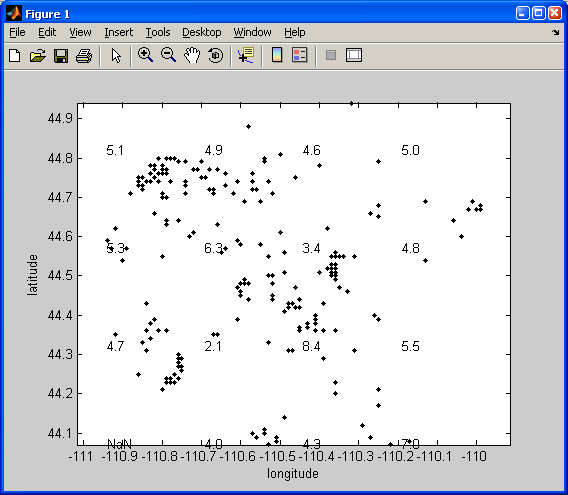
Operations inside the nested loop

stepsize = 0.25;
long_range=min(x_locations):stepsize:max(x_locations);
lat_range = min(y_locations):stepsize:max(y_locations);
for long = long_range
    for lat = lat_range
       tf = x_locations <= long+stepsize./2 & x_locations >= long-stepsize./2 & y_locations <= lat+stepsize./2 & y_locations >= lat-stepsize./2;
       locations = find(tf);
       mean_depth = mean(depth(locations));
       s = sprintf('%2.1f',mean_depth);
       text(long, lat, s);
    end
end

In this example, I have searched for the depth values within each step (+/- half the step size from the lat long location of the estimate). Then, I computed their mean, converted the mean and some text to a string (sprintf), and plotted that amount using text.

3D Plots of Locations - plot3

We could also plot the locations in 3D using the earthquake depth column. Use the plot3 function:

figure(2)
plot3(x_locations,y_locations,-depth,'r.')
grid on
title('Yellowstone Earthquake Hypocenters')
xlabel('longitude')
ylabel('latitude')
zlabel('depth')

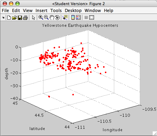
The grid on command is used to display the x,y,z grid in the background to give some perspective to the plot.

Scaled Images of Values in Matrices: using imagesc

We can also gather these values into a matrix that mimics our grid. Then we can plot the scaled values in that matrix using imagesc.

Repeat the last loop, but lets reference the numbers that we loop through in a little bit different way. We will also build out a matrix of our mean depth values.

stepsize = 0.1;
long_range=min(x_locations):stepsize:max(x_locations);
lat_range = min(y_locations):stepsize:max(y_locations);

% Here we are looping over the range of longitudes
for n = 1:length(long_range)

    % Here we are looping over the range of latitudes
    for m = 1:length(lat_range)

        % Notice that we have to index "long_range" by n and "lat_range" by m
        tf = x_locations <= long_range(n)+stepsize./2 & x_locations >= long_range(n)-stepsize./2 & y_locations <= lat_range(m)+stepsize./2 & y_locations >= lat_range(m)-stepsize./2;
        locations = find(tf);

        % Build the "mean_depth" matrix with rows = latitudes, columns = longitudes
        mean_depth(m,n) = mean(depth(locations));
    end
end

Notice some slight changes to our loop.

Lets plot the values of this matrix using imagesc.

The syntax is: imagesc(x,y,D)

This is how we would plot our data:

figure(3)
clf
imagesc(long_range,lat_range,mean_depth)
xlabel('longitude')
ylabel('latitude')
set(gca,'Ydir','normal')
colorbar
hold on

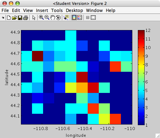
NOTE: The colorbar function will plot the color scale for the image. The set function is used to change Properties after you have plotted your data. Here we change the property, Ydir to plot the y-axis so that larger values are above smaller values. The first argument in set is gca, which tells the set command:"I want to set a property in the current axis (the axis you just plotted your data in)."

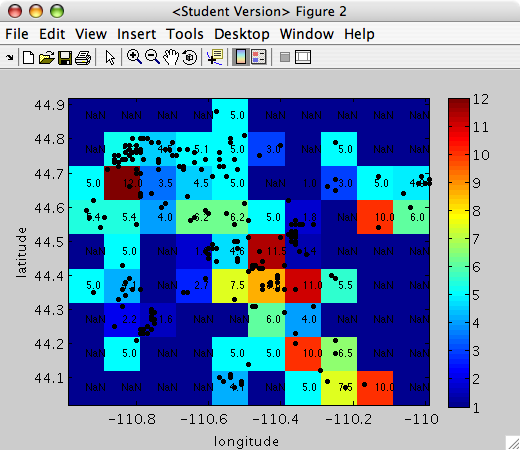
We can then plot the earthquakes over the image, along with the mean depth values in each box:

plot(x_locations,y_locations,'k.')
for n = 1:length(long_range)
    for m = 1:length(lat_range)
        s = sprintf('%2.1f',mean_depth(m,n));
        text(long_range(n), lat_range(m), s);
    end
end

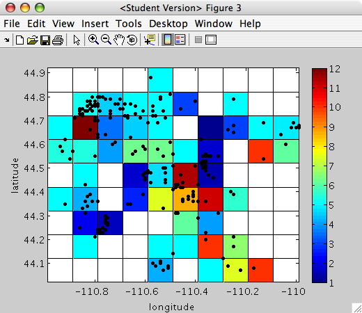
pcolor is similar to imagesc

If you notice the above figure plots grids where there is "no data" (NaN) as blue. This is a limitation of imagesc. The function pcolor plots a pseudocolor image of your matrix. This is very similar to a scaled image produced by imagesc. If you use this function, your "no data" blocks will now be white.

FIRST, we need to precondition our x-axis vector (long_range), y-axis vector (lat_range), and matrix (mean_depth). This is because pcolor plots the colors at the vertices (not the center of the grid like imagesc).

long_range = long_range - (stepsize./2);
lat_range = lat_range - (stepsize./2);
long_range_vert = [long_range (long_range(end)+stepsize)];
lat_range_vert = [lat_range (lat_range(end)+stepsize)];
mean_depth(end+1,:) = NaN .* ones(1,size(mean_depth,2));
mean_depth(:,end+1) = NaN .* ones(size(mean_depth,1),1);

Now we can plot the matrix by replacing imagesc by pcolor:

figure(4)
clf
pcolor(long_range_vert,lat_range_vert,mean_depth)
xlabel('longitude')
ylabel('latitude')
set(gca,'Ydir','normal')
colorbar
hold on
plot(x_locations,y_locations,'k.')

GLG410 Computers in Earth and Space Exploration

Last modified: October 19, 2015

GLG410--Computers in Earth and Space Exploration