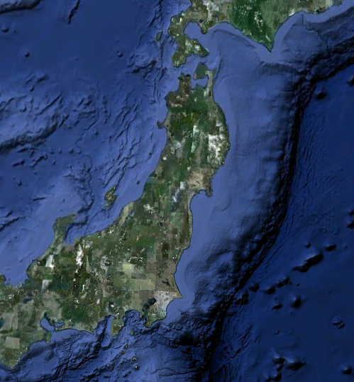
The image drawing is from the upper left and down and to the right. This is called IJ axes. In mapping and other plotting, we may think of the drawing from lower left and up and to the right. This is called XYaxes.
A=imread('http://arrowsmith410-598.asu.edu/Lectures/Lecture16/japan.png');

figure(2)
clf
plot(0,0,'mo')
hold on

for i=1:3
    A(:,:,i)=flipud(A(:,:,i));
end
image(A)
Video explanation:
Now we can register the image to axes that are not simply the pixel positions and display seismicity data on top of it. Here is the Japanese earthquake data to which I am referring and something we have worked on in the past in this course: japaneqs.txt.
A=imread('http://arrowsmith410-598.asu.edu/Lectures/Lecture16/japan.png');


figure(3)
clf
load('japaneqs.txt');
lat = japaneqs(:,1);
long = japaneqs(:,2);

step=0.1;
plot(min(long),min(lat),'m.')
hold on
long_range=min(long):step:max(long);
lat_range=min(lat):step:max(lat);
image(long_range,lat_range,A)

plot(long, lat, 'c.')
Video explanation:
Satellite imagery
Satellite imagery are those images gathered from a satellite platform of the earth.
David has downloaded some ASTER imagery for us and built a nice little script.
Here are the two data files (the HDF file is 124 Mb!): SPCraterASTERData.hdf and SPCraterASTERData.met
First, let's look at the HDFTool:
% Fire up the HDF GUI.
hdftool('SPCraterASTERData.hdf');
Video explanation:
Now let's make an RGB band combination
% ---------------------------- VNIR or CIR --------------------------------
% Pull bands 3N, 2, and 1 from the HDF file into their own matrices. These
% bands are in the VNIR (aka CIR) range and will highlight actively
% photosynthesizing vegetation (showns as red), undisturbed bedrock and
% soils (browns, greens, and greys), and the built environment (blues,
% greens, reddish-purples, and whites)
Band_3 = hdfread('SPCraterASTERData.hdf','VNIR_Swath','Fields','ImageData3N');
Band_2 = hdfread('SPCraterASTERData.hdf','VNIR_Swath','Fields','ImageData2');
Band_1 = hdfread('SPCraterASTERData.hdf','VNIR_Swath','Fields','ImageData1');

% Construct an RGB matrix from the three bands into one 3D matrix.
SPCrater_321 = cat(3,Band_3,Band_2,Band_1);

% Display the image
figure(1)
imshow(SPCrater_321)
xlabel('Longitude (pixels)')
ylabel('Latitude (pixels)')
title('ASTER Bands 3, 2, 1')
One thing you will notice is that the image seems a bit washed out. That is because the colors in the image (values in each of matrices for the bands) are not using the entire display range that is available to them. We can "stretch" the image bands to improve the contrast of the image.
% Perform histogram equalization stretch on the image
for i=1:3
    SPCrater_321_stretch(:,:,i)=histeq(SPCrater_321(:,:,i));
end

% Display the image
figure(2)
imshow(SPCrater_321_stretch)
xlabel('Longitude (pixels)')
ylabel('Latitude (pixels)')
title('ASTER Bands 3, 2, 1 (stretched)')
Let's have a look at a couple more band combinations as we march out to the thermal infrared.
Here is the shortwave infrared (SWIR):
% ---------------------------- SWIR ---------------------------------------
% Pull bands 8, 6, and 4 from the HDF file into their own matrices. These
% bands are in the SWIR range and will highlight spectral features
% diagnostic for iron oxides, illite, kaolinite, and carbonates.
Band_8 = hdfread('SPCraterASTERData.hdf','SWIR_Swath','Fields','ImageData8');
Band_6 = hdfread('SPCraterASTERData.hdf','SWIR_Swath','Fields','ImageData6');
Band_4 = hdfread('SPCraterASTERData.hdf','SWIR_Swath','Fields','ImageData4');

% Construct an RGB matrix from the three bands into one 3D matrix.
SPCrater_864 = cat(3 , Band_8 , Band_6 , Band_4);

% Perform histogram equalization stretch on the image
for i=1:3
    SPCrater_864_stretch(:,:,i)=histeq(SPCrater_864(:,:,i));
end
% Display the image
figure(3)
imshow(SPCrater_864_stretch)
xlabel('Longitude (pixels)')
ylabel('Latitude (pixels)')
title('ASTER Bands 8, 6, 4')
Here is the Thermal Infrared:
% -------------------------- TIR ------------------------------------------
% Pull bands 13, 12, and 10 from the HDF file into their own matrices.
% These bands are in the TIR range and will highlight spectral features
% diagnostic for silicates, iron- and magnesium-bearing minerals and rocks,
% and carbonates. Quartzites are bright red, basaltic rocks are blue,
% granitoids are purple-violet, and carbonates are greenish yellow.
Band_13 = hdfread('SPCraterASTERData.hdf','TIR_Swath','Fields','ImageData13');
Band_12 = hdfread('SPCraterASTERData.hdf','TIR_Swath','Fields','ImageData12');
Band_10 = hdfread('SPCraterASTERData.hdf','TIR_Swath','Fields','ImageData10');

% Construct an RGB matrix from the three bands into one 3D matrix.
SPCrater_131210 = cat(3 , Band_13 , Band_12 , Band_10);

% Do a decorrelation stretch to enhance differences in colors.
SPCrater_131210_decorr = decorrstretch(SPCrater_131210,'Tol',0.01);

% Display the image
figure(4)
imshow(SPCrater_131210_decorr)
xlabel('Longitude (pixels)')
ylabel('Latitude (pixels)')
title('ASTER Bands 13, 12, 10')
Finally, the Normalized Difference Vegetation Index is a single band image derived from mathematical combinations of bands which measure the responce of vegetation very differently. This image is a measure of relative amounts of green vegetation. The NDVI is computed as: (Band_3 - Band_2) ./ (Band_3 + Band_2).
% ---------------------------- NDVI ---------------------------------------
% Compute the Normalized Difference Vegetation Index (NDVI) using the following
% formula: [(Band_3 - Band_2)./(Band_3 + Band_2)]. The NDVI shows the relative
% abundance of actively photosynthesizing vegetation. In other words, it
% assesses how healthy the vegetation is!

% Pull the bands.
Band_3 = hdfread('SPCraterASTERData.hdf','VNIR_Swath','Fields','ImageData3N');
Band_2 = hdfread('SPCraterASTERData.hdf','VNIR_Swath','Fields','ImageData2');
Band_1 = hdfread('SPCraterASTERData.hdf','VNIR_Swath','Fields','ImageData1');

% Calculate NDVI.
% Before we can calculate this, let's look at the format (aka "class" of
% Bands 1, 2, and 3 in the MATLAB Workspace. You will notice that they are
% "uint8", which means they are 8-bit integers! This isn't useful to us,
% especially if we want to do division because division of integers can
% only result in whole numbers. So, we first need to convert these bands to
% a class known as "single" so that we can do some band ratioing!
Band_2 = im2single(Band_2);
Band_3 = im2single(Band_3);
SPCrater_NDVI = (Band_3 - Band_2) ./ (Band_3 + Band_2);

% Display the image.
figure(5)
% Note that because the range of numbers in our NDVI ratio is between
% 0 and 1, we need to display the image's colors using an appropriate scale
% [0 1]
imshow(SPCrater_NDVI,'DisplayRange',[0 1])
xlabel('Longitude (pixels)')
ylabel('Latitude (pixels)')
title('NDVI computed from ASTER Image')
In this assignment, you will follow along the examples from this lecture with respect to processing ASTER images and apply it to a new dataset covering the Phoenix area.
The ASTER HDF file is here: PhoenixASTERData.hdf
Download this to your Matlab ASTER directory and modify your practice scripts that you have built following along the lecture and produce 4 figures: CIR, SWIR, TIR, and NDVI for the area. Export the figures as jpeg (use the same print -djpeg command that you have used before). Zoom into an area of interest and you can save those zooms from the menu bar on the figure (File->Save as->Save as type jpeg). Note that this means you will be submitting 8 images: 4 will be the entire extent of the images you have produced and the other 4 will be of the zoom areas (they don't have to be the same target--choose places that help illustrate that you understand how the various band combinations are showing the surface properties).
Provide your commented script and any functions you build along with your images as a web page linked from your assignments page.
In addition, write a short paragraph that compares and contrasts how the four image band combinations displays the variable GEOLOGY, URBAN features, and VEGETATION in the area.
This assignment is due Wednesday, October 28 by the beginning of class.