| Announcements | Syllabus | Schedule | Weekly lecture notes | Assignments | Links |
Matlab is a program that has been developed for the general solution of mathematical equations, data processing, and data display. MATLAB is an acronym for MATrix LABoratory and it is a highly optimized numerical computation and matrix manipulation package. It is an excellent tool for developing numerical models of problems, performing mathematical operations on large data sets, displaying data in one, two, three, or four dimensions, and solving simultaneous equations. In general, Matlab has been developed as a numerical tool and so best works on real numbers, rather than symbolic operations.
Matlab is a product of The Mathworks. Cleve Moler is the inventor of Matlab and a founder of Matlab.
In short, if you can write an equation that you think represents a relationship between two or more variables and need to graph your results, Matlab is the tool to use. First, we will go through a short introduction on Matlab concepts, entry formats, graphics, M-files, and functions.
As a similar but open source and free alternative, you may wish to install and run the software package "R": https://www.r-project.org/. It has similar capabilities and similar syntax, etc. But, you don't need to do this as long as you are an ASU student because you have good access to Matlab. Look towards the bottom of this lecture to see a video about running MATLAB on ASU MyApps.
Copy and paste this into the Matlab command line: playbackdemo('GettingStartedwithMATLAB', 'toolbox/matlab/demos/html')
NOTE: For multiplication, division, and exponents, remember to use the dot (.) BEFORE the math symbol. This is not necessarily needed all the time, but is good practice to use it anyway to avoid problems with vector and matrix operations in the future.Addition (+)
>> 4 + 7

ans =

    11
Subtraction (-)
>> 48 - 8.2

ans =

    39.8
Multiplication (.*)
>> 4.53 .* 6

ans =

    27.18
Division (./)
>> 200 ./ 50

ans =

    4
Exponents (.^)
>> 4.1 .^ 3

ans =

    68.921
Trig Functions in Radians (sin, cos, tan, sec, cot, csc)
>> sin(0.8)

ans =

    0.71736
Trig Function in Degrees (sind, cosd, tand, secd, cotd, cscd)
>> sind(90)

ans =

    1
Inverse Trig Functions in Radians (asin, acos, atan, atan2, asec, acot, acsc)
>> acos(0.567)

ans =

    0.96794
Inverse Trig Functions in Degrees (asind, acosd, atand, asecd, acotd, acscd)
>> acosd(0.5)

ans =

    60
Square Roots
>> sqrt(16)

ans =

    4
Exponentials
>> exp(2.3)

ans =

    9.9742
Natural Logarithms
>> log(456384)

ans =

    13.031
Base 10 Logarithms (this is special)
>> log10(10000)

ans =

    4
Absolute Value
>> abs(-31.45)

ans =

    31.45
There are a few special numbers that are important to know. Some you will use all the time, some not so much.>> pi
ans =
3.1416
Imaginary (Complex) Numbers
>> i

ans =

    0 +    1i
Not-a-Number (this acts like a place holder for a value, except it has no value)
>> NaN

ans =

    NaN
Infinity
>> inf

ans =

    Inf
Smallest incremental number (the precision of the computer)
>> eps

ans =

    2.2204e-16
Combining operations - using parenthesis ()>> 2 .* pi ./ 360 .* 6371 .* sind(90 - 43.8)
ans =

    80.256
REMEMBER YOUR "ORDER OF OPERATIONS"!! I recommend using parenthesis for EVERY separate operation to organize your equations. A common source of error is either forgetting to close parenthesis (easily corrected), or putting parenthesis in the wrong place (hard to find and correct!).>> (2 .* pi ./ 360 .* 6371 .* sind(90 - 43.8)
??? (2 .* pi ./ 360 .* 6371 .* sind(90 - 43.8)
|
Error: Expression or statement is incorrect--possibly unbalanced (, {, or [.
Oops! I forgot to close a parenthesis. Let's try it again.>> ((2 .* pi) ./ 360) .* (6371 .* sind(90 - 43.8))
ans =
80.256
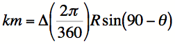
This time I grouped the parts of the equation that make sense. For full disclosure, this particular equation is for converting degrees of Longitude to kilometers around a given line of Latitude.
ans =
80.256
Matlab is assigning your answer to a default variable called ans. Every time you do a calculation in Matlab, ans is replaced in the Workspace window.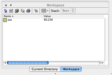
>> kilometers = ((2 .* pi) ./ 360) .* (6371 .* sind(90 - 43.8))You will notice that Matlab has been echoing your output by saying:
kilometers =

    80.256
Now we can use this variable in another equation. Lets just say we want to convert the kilometers to miles.
>> miles = kilometers .* 0.62137

miles =

    49.869
SEMICOLONS>> kilometers = ((2 .* pi) ./ 360) .* (6371 .* sind(90 - 43.8));Naming Conventions/Suggests (Any Programming Language)
>> RowVector = [1 2 3 4 5 6 7 8 9 10];
>> RowVector

RowVector =

    1 2 3 4 5 6 7 8 9 10
Column Vector
>> ColumnVector = [1; 2; 3; 4; 5; 6; 7; 8; 9; 10];
>> ColumnVector

ColumnVector =

    1
    2
    3
    4
    5
    6
    7
    8
    9
    10
Matrix (2 x 5)
>> Matrix = [1 2; 3 4; 5 6; 7 8; 9 10];
>> Matrix

Matrix =

    1  2
    3  4
    5  6
    7  8
    9  10
Array Operations
>> Matrix = Matrix .* 2;
>> Matrix

Matrix =

    2  4
    6  8
    10  12
    14  16
    18  20
>> RowVector(3)

ans =

    3

>> ColumnVector(4)

ans =

    4
Array Indexing (matrices)
>> Matrix(3,2)

ans =

    6
NOTE: Rows are referenced first, then columns.Array Indexing (entire row or column)
>> Matrix(3,:)

ans =

    5  6
Rules to Remeber
>> Name = 'My name is Kevin';
>> Name

Name =

My name is Kevin
This is a 16-element array.
>> load('SRDischarge2008.txt','-ascii');
The first argument in the load function is the filename. The second argument is the file type. In the case of a text file, it is always '-ascii'.>> min(SRDischarge2008(:,2))
ans =
0
Maximum Value (2nd column - discharge)
>> max(SRDischarge2008(:,2))

ans =

    5900
Average or Mean Value (2nd column - discharge)
>> mean(SRDischarge2008(:,2))

ans =

    5900
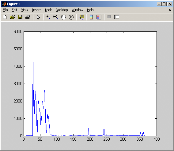
>> plot(SRDischarge2008(:,1),SRDischarge2008(:,2));The first argument is the x-axis values. The second argument is the y-axis values. (NOTE: These MUST BE the same length!)
>> title('Salt River Discharge at Priest Dr. - 2008');
X-Axis Label
>> xlabel('Day of Year');
Y-Axis Label
>> ylabel('Daily Discharge (cfs)');
Now what do we have.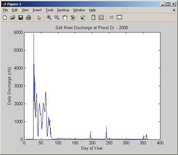
NOTE: You can also play around with the plot using buttons and functions within the Figure Window.Saving a graph to a JPEG is very helpful for placing this graph in the context of a report (or maybe your homework). To save a figure, you will use the print function. Here is how to do it:
>> print('discharge.jpg','-djpeg');
The first argument is the filename of the JPEG image. The second argument ('-djpeg') tells Matlab that you are saving it in JPEG format.>> saveThe default filename for your saved workspace is "matlab.mat". If you want to save it under a different name, you add that name as an argument to the function.
>> save('lecture3.mat');
NOTE: This will ONLY save the variables in your workspace. It DOES NOT save figures or plots that you have made.To load in a saved MAT-file, you will use the load function, similar to what we did with the text files.
>> load('lecture3.mat','-mat');
The first argument in the filename. The second argument is the format of the file you are wanting to load. For MAT-files, this is always '-mat'. (NOTE: In this case, the second argument is optional because '-mat' is the default choice.)